Virtual Screening for Protein-Ligand Binding Sites: Principles, Methods, and Best Practices in Modern Drug Discovery

Abstract

This article provides a comprehensive overview of virtual screening (VS) for identifying protein-ligand binding sites, a cornerstone of modern computational drug discovery. Aimed at researchers, scientists, and drug development professionals, it covers foundational principles, exploring the core concepts of ligand-based and structure-based approaches. The scope extends to detailed methodological applications, including docking, pharmacophore modeling, and emerging machine learning techniques. It critically addresses common challenges and troubleshooting strategies, emphasizing protocol validation to avoid false positives. Finally, the article examines rigorous validation standards and comparative performance of different methods, including insights from blinded community challenges. The synthesis of these four intents provides a holistic guide for designing effective and reliable virtual screening workflows to accelerate lead identification and optimization.

The Foundations of Virtual Screening: Core Concepts and Strategic Goals

Virtual screening (VS) represents a cornerstone of modern computational drug discovery. It encompasses a set of in silico techniques used to evaluate massive libraries of chemical compounds and identify those with the highest potential to bind to a therapeutic protein target and modulate its biological function [1]. By leveraging computational power, VS addresses a fundamental challenge in drug discovery: efficiently navigating the vastness of chemical space to find promising starting points for drug development, thereby reducing the costs and time associated with experimental high-throughput screening (HTS) alone [2] [1].

The primary purpose of virtual screening is library enrichment—sifting through thousands to billions of compounds to select a much smaller subset enriched with putative active molecules [3]. This process enables researchers to focus their experimental efforts on the most promising candidates, dramatically improving research efficiency. A more focused application involves compound design, where detailed analysis of smaller compound series guides the optimization of lead molecules, ideally with quantitative predictions of binding affinity [3].

The Virtual Screening Paradigm: Ligand-Based and Structure-Based Approaches

Virtual screening methodologies are broadly classified into two complementary categories: ligand-based and structure-based methods. The choice between them often depends on the availability of prior knowledge about either known active compounds or the three-dimensional structure of the target protein.

Ligand-Based Virtual Screening (LBVS)

LBVS methods do not require a 3D structure of the target protein. Instead, they leverage the chemical information from known active ligands to identify new hits with similar structural or pharmacophoric features [3]. The core assumption is that structurally similar molecules are likely to exhibit similar biological activities.

• Molecular Similarity and Fingerprints: This approach involves computing molecular fingerprints, such as MACCS keys or ECFP4, for known active compounds and then screening large databases to find compounds with high similarity, typically measured by the Tanimoto coefficient [4]. This method is computationally fast and excellent for pattern recognition across diverse chemistries [3].
• Pharmacophore Modeling: A pharmacophore represents the essential spatial and electronic functional arrangements necessary for a molecule to interact with a biological target. Pharmacophore models can be generated from a set of active ligands or from a protein binding site if known. These models are then used as 3D queries to screen compound libraries [4].
• Quantitative Structure-Activity Relationship (QSAR): Advanced methods like Quantitative Surface-field Analysis (QuanSA) construct physically interpretable binding-site models based on ligand structure and affinity data using multiple-instance machine learning. These can predict both ligand binding pose and quantitative affinity, providing valuable resolution for compound design [3].

Structure-Based Virtual Screening (SBVS)

SBVS relies on the three-dimensional structure of the target protein, obtained through experimental methods like X-ray crystallography or cryo-electron microscopy, or via computational predictions [3]. The most common SBVS technique is molecular docking.

• Molecular Docking: This process involves computationally predicting the preferred orientation (pose) of a small molecule when bound to a protein target. The workflow typically consists of two components: pose generation, which explores different conformations and orientations of the ligand within the binding site, and scoring, which ranks these poses based on an estimated binding affinity using a scoring function [5] [4].
• Absolute Binding Free Energy Calculations: Protocols like Absolute Binding FEP+ (ABFEP+) represent the state-of-the-art for affinity prediction. They provide highly accurate calculations of binding free energies but are computationally very demanding, typically limiting their application to smaller sets of compounds [2].
• Handling Protein Flexibility: Advanced docking protocols, such as RosettaVS, incorporate receptor flexibility by allowing side-chain and limited backbone movement, which is critical for accurately modeling induced conformational changes upon ligand binding [5].

The Hybrid Approach: Combining LBVS and SBVS

Integrating ligand-based and structure-based methods often yields more reliable results than either approach alone [3]. Two common integration strategies are:

• Sequential Workflows: A rapid ligand-based filter (e.g., molecular similarity) is first applied to a large compound library to identify a promising subset. This subset then undergoes more computationally expensive structure-based refinement through docking [1] [3]. This conserves resources while improving precision.
• Parallel Screening and Consensus Scoring: Ligand- and structure-based screenings are run independently on the same library. Results are then combined through consensus scoring frameworks, which can either select top candidates from both lists or create a unified ranking by averaging scores. This strategy mitigates the limitations inherent in each method and increases confidence in selecting true positives [4] [3].

A Detailed Protocol for a Modern Virtual Screening Workflow

The following section outlines a robust, modern VS workflow that integrates both ligand- and structure-based methods, suitable for screening ultra-large chemical libraries.

Stage 1: Target Preparation and Binding Site Identification

Objective: To define a high-quality protein structure and its relevant ligand-binding pocket.

• Target Protein Selection and Structure Sourcing: The target protein is selected based on its therapeutic relevance. A 3D structural model is then acquired.
  • Sources: The Protein Data Bank (PDB) is the primary source for experimental structures [1]. For targets with no solved structure, computationally predicted models from AlphaFold2 can be used [6] [1]. Users should evaluate per-residue confidence scores (pLDDT) to assess local model quality, especially in the binding region [1].
• Structure Preparation: Using software like Molecular Operating Environment (MOE) or ChimeraX, the protein structure is prepared by:
  • Removing water molecules and extraneous ligands.
  • Adding hydrogen atoms and assigning appropriate atom charges (e.g., using the AMBER10_EHT forcefield) [4].
  • Minimizing the structure to relieve steric clashes.
• Binding Site Identification: The ligand-binding site must be defined for docking.
  • Preferred Method: If the site is known from literature or mutation studies, coordinates can be defined based on a co-crystallized ligand or conserved residues [1].
  • Computational Prediction: If the site is unknown, use pocket detection algorithms like Fpocket [1], ConCavity, or 3DLigandSite [7]. Using multiple algorithms is encouraged for consensus [1].

Stage 2: Library Preparation and Initial Triage

Objective: To prepare a library of synthesizable small molecules and apply rapid filters to reduce its size.

• Library Curation: Compile a library of compounds for screening. These can be commercial vendor libraries, in-house collections, or enormous synthetically accessible spaces like Enamine REAL containing billions of molecules [2]. Canonical SMILES codes are typically used as the standard molecular representation.
• Prefiltering: The library is filtered based on physicochemical properties (e.g., molecular weight, lipophilicity) to remove compounds with undesirable drug-like or lead-like properties [2]. Additionally, tools like SwissADME can be used to flag pan-assay interference compounds (PAINS) and predict ADMET (Absorption, Distribution, Metabolism, Excretion, and Toxicity) profiles [4].

Stage 3: Active Learning-Guided Docking

Objective: To efficiently screen billions of compounds by docking only the most promising candidates.

• Machine Learning-Guided Docking: For ultra-large libraries, brute-force docking is computationally prohibitive. Instead, active learning protocols like AL-Glide are employed [2]. This method iteratively trains a machine learning model on a small subset of docked compounds. The model learns to predict docking scores and prioritizes the next batch of compounds for docking, dramatically reducing the number of full docking calculations required.
• High-Throughput Docking: The top-ranked compounds from the active learning step (e.g., 10-100 million) are subjected to a full docking calculation using programs like Glide [2], AutoDock Vina, or RosettaVS [5] [1]. At this stage, a standard docking protocol with a rigid receptor is often sufficient.

Stage 4: Rescoring and Hit Prioritization

Objective: To refine the ranking of top hits from the initial docking screen using more accurate, computationally intensive methods.

• Pose Refinement and Rescoring: The best-scoring compounds from initial docking are redocked and scored using more sophisticated methods. Glide WS (WaterScore), for example, uses explicit water information for more accurate pose prediction and scoring [2]. The RosettaVS protocol uses a high-precision (VSH) mode that includes full receptor flexibility [5].
• Absolute Binding Free Energy Calculations: The most promising few hundred to thousand compounds can be subjected to rigorous Absolute Binding FEP+ (ABFEP+) calculations [2]. This physics-based method provides highly accurate binding affinity predictions and is a linchpin for selecting the most potent compounds.
• Consensus Scoring and MPO: Finally, a consensus approach is used to prioritize hits. This can combine scores from different methods (e.g., docking scores, FEP+ predictions, ligand-based similarity scores) [3]. The final list is then evaluated through Multi-Parameter Optimization (MPO), which balances predicted affinity with other critical properties like selectivity, ADME, and safety to identify the overall best candidates for experimental testing [3].

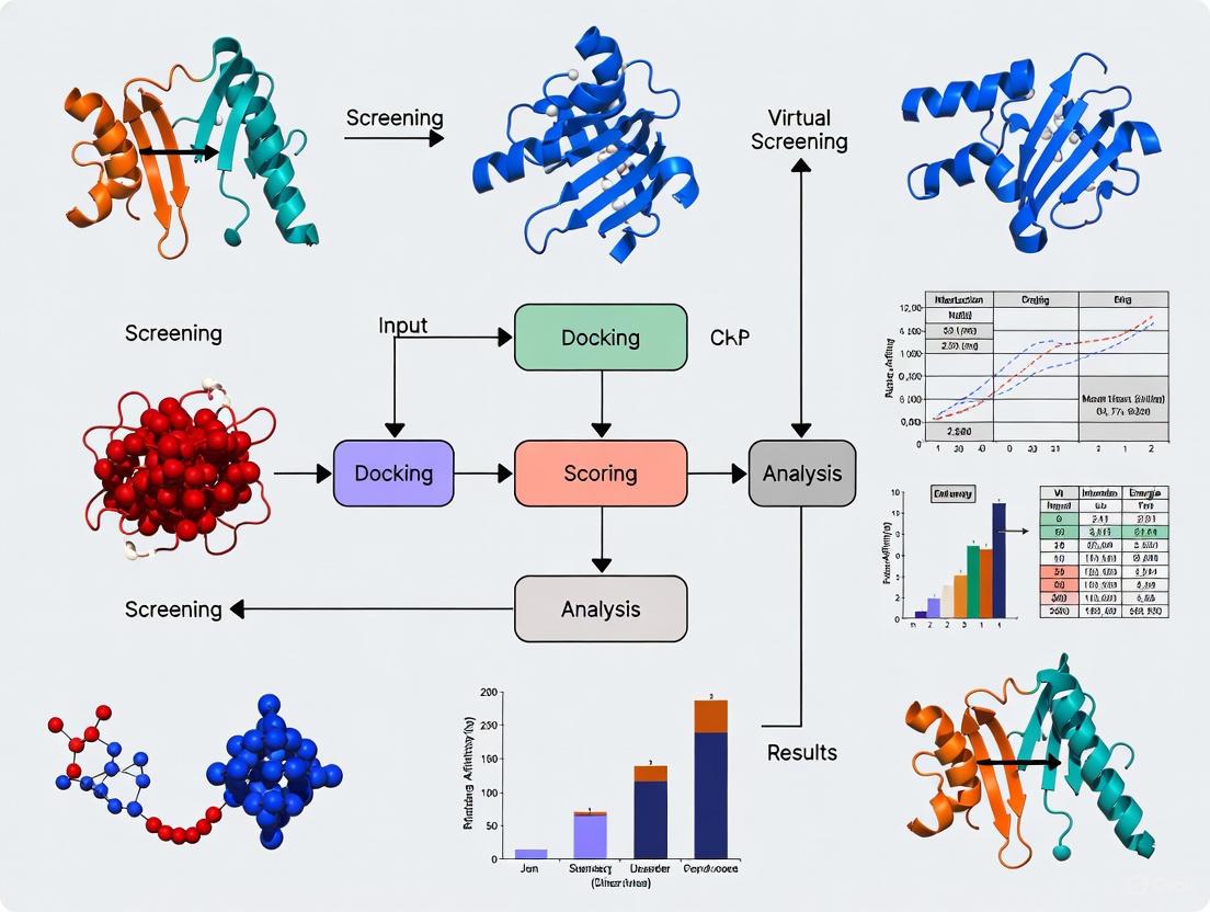
The following workflow diagram synthesizes this multi-stage protocol into a coherent, actionable pathway.

Virtual Screening Workflow

Performance Benchmarks and Impact

Modern VS workflows have demonstrated a dramatic improvement in hit rates compared to traditional methods. Schrödinger's Therapeutics Group reported that their modern VS workflow, leveraging ultra-large scale docking and ABFEP+ calculations, consistently achieved double-digit hit rates across multiple projects and diverse protein targets [2]. This is a significant increase from the typical 1-2% hit rates observed with traditional VS approaches.

Performance on standard benchmarks further validates these advanced methods. On the CASF2016 benchmark, the RosettaGenFF-VS scoring function achieved a top 1% enrichment factor (EF1%) of 16.72, significantly outperforming the second-best method (EF1% = 11.9) [5]. This indicates a superior ability to identify true binders early in the ranked list. Furthermore, Ligand-Transformer, a deep learning method, demonstrated strong correlation with experimentally measured binding affinities (Pearson’s R value of 0.57), which increased to 0.88 after fine-tuning on a specific target dataset [6].

The following table summarizes key performance metrics from recent studies:

Table 1: Performance Benchmarks of Modern Virtual Screening Methods

Method / Platform	Key Metric	Result / Performance	Context / Dataset
Schrödinger VS Workflow [2]	Experimental Hit Rate	Double-digit hit rates (e.g., >10%)	Multiple diverse protein targets
RosettaGenFF-VS [5]	Enrichment Factor (Top 1%)	16.72	CASF-2016 Benchmarking Dataset
Ligand-Transformer [6]	Affinity Prediction Correlation (R)	0.57 (0.88 after fine-tuning)	PDBbind2020 and EGFRLTC-290 datasets
Drugsniffer Pipeline [1]	Screening Throughput	~40,000 compute hours for 3.7B molecules	Three SARS-CoV-2 protein targets

A successful virtual screening campaign relies on a suite of software tools and databases. The table below catalogs key resources, categorizing them by their primary function in the workflow.

Table 2: Essential Research Reagents and Computational Tools

Category	Tool / Resource	Primary Function & Description
Protein Structure Databases	Protein Data Bank (PDB) [1]	Primary repository for experimentally determined 3D structures of proteins and nucleic acids.
	AlphaFold Protein Structure Database [1]	Database of protein structure predictions generated by the AlphaFold2 AI system.
Binding Site Detection	Fpocket [7] [1]	An open source protein pocket detection algorithm based on Voronoi tessellation and alpha spheres.
	ConCavity [7]	Predicts binding sites by integrating evolutionary sequence conservation and 3D structural information.
Compound Libraries	Enamine REAL [2]	An ultra-large library of billions of readily synthesizable compounds.
	BIOFACQUIM [4]	A publicly available database of natural products and semi-synthetic compounds isolated and/or designed in Mexico.
Ligand-Based Screening	RDKit [4]	Open-source cheminformatics toolkit used for fingerprint generation, similarity calculations, and molecular operations.
	ROCS [3]	A tool for rapid 3D shape-based superposition and screening to find molecules with similar shape and chemistry.
Structure-Based Docking	Glide [2] [5]	A high-performance docking tool for predicting protein-ligand binding modes and scoring.
	AutoDock Vina [5] [1]	A widely used, open-source docking program known for its speed and accuracy.
	RosettaVS [5]	An open-source docking and VS protocol that allows for receptor flexibility and uses the RosettaGenFF-VS force field.
Advanced Scoring & FEP	Absolute Binding FEP+ (ABFEP+) [2]	A state-of-the-art protocol for calculating absolute binding free energies with high accuracy.
Workflow & Automation	Drugsniffer [1]	An open-source, massively-scalable pipeline that integrates LBVS and SBVS for screening billions of molecules.
	VirtualFlow [1]	An open-source platform designed for ultra-large virtual screening campaigns on high-performance computing clusters.

Virtual screening has evolved from a supplementary tool to a critical driver in drug discovery. The integration of ligand-based and structure-based methods, coupled with machine learning acceleration and rigorous physics-based scoring, now enables researchers to reliably identify high-quality, potent hits from libraries of billions of compounds. The standardized workflows and robust benchmarks outlined in this document provide a framework for researchers to conduct effective virtual screening campaigns. As computational power and methodologies continue to advance, VS will play an increasingly pivotal role in accelerating the delivery of new therapeutics.

Ligand-Based Virtual Screening (LBVS) is a foundational computational technique in modern drug discovery, employed when the three-dimensional structure of a biological target is unknown or unavailable. Operating on the principle that molecules with similar structural or physicochemical properties are likely to exhibit similar biological activities, LBVS uses known active compounds as templates to identify new hit molecules from vast chemical libraries [8] [9]. This approach stands in contrast to structure-based methods, which rely on the target's 3D structure, and is particularly valuable for targets like G-protein-coupled receptors (GPCRs) or proteins where obtaining a high-resolution structure is challenging [8] [10]. The core of LBVS involves two essential components: a robust method for quantifying molecular similarity and a reliable scoring function to rank database compounds, enabling the effective discrimination of active from inactive molecules [8]. This Application Note provides a detailed overview of LBVS methodologies, supported by quantitative performance data, step-by-step experimental protocols, and practical toolkits for implementation, framed within the broader context of virtual screening for protein-ligand binding site research.

Key Methodologies and Performance Metrics

Ligand-based virtual screening encompasses a range of techniques, from simple 2D similarity searches to complex 3D shape and field comparisons. The choice of method often depends on the available ligand information and the desired balance between computational speed and accuracy.

Table 1: Core LBVS Methodologies and Their Characteristics

Methodology	Molecular Representation	Similarity Measure	Key Advantages	Common Tools/Examples
2D Fingerprint	Bit vectors encoding structural fragments	Tanimoto, Dice, Cosine	High speed, suitable for ultra-large libraries [11]	ECFP, FCFP, RDKit [11]
Pharmacophore	3D arrangement of chemical features	Pattern matching	Incorporates chemical functionality logic [9]	Catalyst, Phase [9]
Shape-Based	Molecular volume/van der Waals surface	Volume overlap (e.g., Tanimoto)	Identifies scaffolds with similar shape but different chemistry [8] [9]	ROCS, VSFlow [8] [11]
Field-Based	Electrostatic, hydrophobic properties	Field similarity	Accounts for key interaction forces [9]	FieldScreen [9]
Graph-Based	Attributed graphs (nodes/edges as features)	Graph Edit Distance (GED)	Directly uses molecular topology, high interpretability [12]	Custom algorithms [12]

The performance of LBVS approaches is quantitatively evaluated using several standard metrics derived from enrichment studies. These metrics assess a method's ability to prioritize active compounds early in the ranked list.

Table 2: Quantitative Performance of LBVS Methods on Benchmark Datasets

Method / Score	Dataset / Context	Performance Metric	Result / Enrichment
HWZ Score [8]	40 targets from DUD	Average AUC	0.84 ± 0.02
HWZ Score [8]	40 targets from DUD	Hit Rate at top 1%	46.3% ± 6.7%
HWZ Score [8]	40 targets from DUD	Hit Rate at top 10%	59.2% ± 4.7%
BINRF Model [13]	Structurally heterogeneous MDDR classes	Retrieval effectiveness	Significant improvement vs. baseline
Graph Edit Distance [12]	Multiple public datasets (e.g., DUD-E, MUV)	Classification accuracy	Highest ratios in bioactivity similarity

Detailed Experimental Protocols

Protocol 1: LBVS Workflow Using the VSFlow Toolkit

VSFlow is an open-source, command-line tool that integrates multiple LBVS methods, making it an excellent platform for standardized screening campaigns [11].

1. Database Preparation:

• Input: A compound library in SDF, SMILES, or other common formats.
• Standardization: Run preparedb with the -standardize flag to apply MolVS rules, which include charge neutralization, salt removal, and optional tautomer canonicalization [11].
• Conformer Generation: For 3D screenings, use the -conformers flag to generate multiple conformers for each database molecule using the RDKit ETKDGv3 method. Optimize conformers with the MMFF94 force field.
• Fingerprint Calculation: Use the -fingerprint flag to generate and store molecular fingerprints (e.g., ECFP4) within the database for fast 2D searches.
• Output: A dedicated, high-speed .vsdb database file for subsequent screening.

2. Screening Execution:

• Substructure Search: Use the substructure tool with a SMARTS pattern query. The tool uses RDKit's GetSubstructMatches() to find all molecules containing the specified substructure.
• Fingerprint Similarity Search: Use the fpsim tool with a query molecule (SMILES) and a chosen fingerprint (e.g., Morgan fingerprint with 2048 bits and radius 2). The Tanimoto coefficient is a default similarity measure. The -simmap parameter can be added to generate a similarity map visualizing contributing atoms.
• Shape-Based Screening: Use the shape tool. The query molecule's conformers are aligned against all conformers of each database molecule using RDKit's Open3DAlign. Shape similarity (e.g., TanimotoDist) and 3D pharmacophore fingerprint similarity are calculated. A combined score (average of shape and pharmacophore similarity) is used to rank the results [11].

3. Results Analysis and Visualization:

• VSFlow can output results in various formats (SDF, Excel, CSV, PDF). The PDF output provides a convenient table of hits with 2D structures and highlighted substructure matches.

Protocol 2: Bayesian Inference Network with Reweighting

This protocol is designed for multi-reference similarity searching, especially effective for structurally heterogeneous active sets [13].

1. System Setup and Fingerprint Generation:

• Convert the molecular database (e.g., MDL Drug Data Report (MDDR)) and the set of known active reference structures into folded fingerprint vectors (e.g., 1024-element ECFC_4 fingerprints).

2. Fragment Reweighting:

• For each fragment i in the fingerprint, calculate a reweighting factor rwf_i based on its frequency in the set of active references [13]: rwf_i = F_fi / maxF where F_fi is the frequency of the fragment in the reference set and maxF is the maximum fragment frequency in that set.
• Calculate a new weight nw_i for each fragment: nw_i = w_i + rwf_i where w_i is the original frequency of the fragment in a single reference structure. This process amplifies the importance of fragments common across many active molecules.

3. Network Execution and Ranking:

• Implement a Bayesian inference network with three node types: compound nodes (root), fragment nodes, and a reference structure node (leaf).
• Calculate the belief in each fragment node using a function like the Okapi belief function, incorporating the new fragment weights nw_i.
• The belief in the reference node is computed by aggregating the beliefs from its parent fragment nodes. The final belief score reflects the probability of a database compound having similar bioactivity to the reference set.
• Rank all database compounds in decreasing order of this probability score for experimental validation.

Workflow Visualization

LBVS Decision and Execution Workflow

The Scientist's Toolkit: Essential Research Reagents & Solutions

Table 3: Key Software Tools and Resources for LBVS

Tool / Resource	Type / Availability	Primary Function in LBVS	Application Note
VSFlow [11]	Open-source command-line tool	Integrated 2D/3D ligand-based screening	Allows customizable substructure, fingerprint, and shape-based screening from a unified interface.
RDKit [11]	Open-source cheminformatics library	Core chemistry engine	Provides foundational functions for molecule handling, fingerprint generation, and conformer generation used by many tools.
ROCS [8] [9]	Commercial software	Rapid 3D shape-based screening	Industry standard for shape and chemical overlay; uses Gaussian functions for molecular volume.
Database of Useful Decoys (DUD/DUD-E) [8] [12]	Public benchmark dataset	Method validation and benchmarking	Provides target-specific sets of known actives and property-matched decoys for retrospective VS performance tests.
MDDR Database [13]	Commercial activity database	Source of known active compounds	Used for building and testing similarity search models against pharmaceutically relevant targets.
SwissSimilarity [11]	Free web server	2D/3D screening of public & vendor libraries	Provides easy access to similarity searching without local installation, useful for initial explorations.
Tenuifoliside B	Tenuifoliside B, CAS:139726-36-6, MF:C30H36O17, MW:668.6 g/mol	Chemical Reagent	Bench Chemicals
Deltatsine	Deltatsine, CAS:92631-66-8, MF:C25H41NO7, MW:467.6 g/mol	Chemical Reagent	Bench Chemicals

Ligand-based virtual screening remains a powerful and efficient strategy for hit identification in the absence of a protein structure. Its success is anchored in the careful selection of molecular representation and similarity metrics, as evidenced by the strong performance of modern shape-based and graph-based methods on standardized benchmarks. The availability of robust, open-source toolkits like VSFlow lowers the barrier to entry for implementing these protocols. When integrated into a broader drug discovery workflow—either as a primary screening method or in a hybrid approach combining ligand- and structure-based insights—LBVS significantly accelerates the identification of novel, promising scaffolds for further optimization.

Structure-Based Virtual Screening (SBVS) is a cornerstone of modern computer-aided drug design (CADD), functioning as a computational technique to identify novel drug candidates by predicting how small molecules interact with a three-dimensional protein target [14]. The core principle involves molecular docking, which computationally simulates the binding of a ligand to a protein receptor, predicting the stable conformation of the complex and its binding affinity [15]. This process is fundamental to understanding protein-ligand interactions, which are driven by non-covalent forces such as hydrogen bonds, ionic interactions, van der Waals forces, and hydrophobic effects [14]. By leveraging the known 3D structure of a protein, SBVS allows researchers to rapidly prioritize compounds with a high likelihood of binding from immense chemical libraries, significantly accelerating the pace of early-stage drug discovery and providing crucial mechanistic insights for rational drug design [14] [16].

Key Principles of Molecular Docking

Physicochemical Basis of Binding

Protein-ligand binding is a complex process governed by non-covalent interactions and thermodynamics. The formation of a stable protein-ligand complex is driven by a favorable change in the Gibbs free energy of binding (ΔG_bind), which is determined by the enthalpy (ΔH) from the formation of chemical bonds and the entropy (ΔS) related to the system's randomness [14]. The key non-covalent interactions that contribute to binding include:

• Hydrogen Bonds: Polar electrostatic interactions between a hydrogen atom donor and an acceptor, with a strength of approximately 5 kcal/mol. They are highly specific and crucial for biomolecular recognition [14].
• Ionic Interactions: Electrostatic attractions between oppositely charged ionic pairs, providing highly specific binding forces within the protein's binding pocket [14].
• Van der Waals Interactions: Non-specific forces arising from transient dipoles in electron clouds when atoms are in close proximity, with weaker strength of about 1 kcal/mol [14].
• Hydrophobic Interactions: Entropy-driven associations where nonpolar molecules or regions aggregate to minimize disruptive interactions with the aqueous solvent [14].

Molecular Recognition Models

The mechanisms by which proteins and ligands recognize and bind to each other are conceptualized through three primary models:

• Lock-and-Key Model: Proposes that the binding partners are pre-complementary in shape, with rigid interfaces that fit perfectly without conformational changes. This model represents an entropy-dominated process [14].
• Induced-Fit Model: Suggests that the protein binding site undergoes conformational adjustments to accommodate the ligand, adding flexibility to the original lock-and-key hypothesis [14].
• Conformational Selection Model: Postulates that ligands selectively bind to pre-existing conformational states from an ensemble of protein substates, with the population of the selected state increasing upon binding [14].

Table 1: Fundamental Interactions in Protein-Ligand Binding

Interaction Type	Strength (kcal/mol)	Nature	Role in Binding
Hydrogen Bonds	~5	Electrostatic, directional	Specificity and stability
Ionic Interactions	5-10	Electrostatic, charged	Strong, specific attraction
Van der Waals	~1	Non-specific, transient	Close-contact stabilization
Hydrophobic Effect	Variable	Entropy-driven	Burial of non-polar surfaces

Current Methodologies and Tools

The SBVS landscape encompasses both traditional physics-based approaches and emerging deep learning methods, each with distinct strengths and applications.

Traditional Docking Approaches

Traditional docking tools like AutoDock Vina and Glide SP employ scoring functions based on empirical or physics-based energy terms to evaluate binding poses, combined with search algorithms to explore the conformational space [15]. These methods have proven robust and reliable, with Glide SP particularly noted for producing physically plausible poses with high validity rates (above 94% across benchmark datasets) [15].

Deep Learning-Enhanced Docking

Recent advances in artificial intelligence have introduced several paradigms that are transforming the docking field [15]:

• Generative Diffusion Models (e.g., SurfDock): Demonstrate superior pose prediction accuracy, achieving RMSD ≤ 2Ã… success rates exceeding 70% across diverse datasets [15].
• Regression-Based Models: Directly predict binding affinities or poses but often struggle with producing physically valid conformations [15].
• Hybrid Methods: Combine traditional conformational searches with AI-driven scoring functions, offering a balanced approach between accuracy and physical plausibility [15].

Table 2: Performance Comparison of Docking Methodologies

Method Category	Representative Tools	Pose Accuracy (RMSD ≤ 2Å)	Physical Validity (PB-valid)	Best Use Case
Traditional Docking	Glide SP, AutoDock Vina	Moderate to High	High (≥94%)	Standard docking with high physical plausibility
Generative Diffusion	SurfDock, DiffBindFR	High (≥70%)	Moderate (40-63%)	Maximum pose accuracy
Regression-Based	KarmaDock, QuickBind	Variable	Low to Moderate	Rapid screening when speed is critical
Hybrid Methods	Interformer	Moderate	Moderate to High	Balanced approach for diverse targets

Integrated Screening Platforms

Modern drug discovery increasingly utilizes multi-stage platforms that combine multiple methodologies:

• HelixVS: Implements a three-stage workflow combining classical docking (AutoDock QuickVina 2) with deep learning-based affinity scoring (RTMscore) and optional binding mode filtering. This approach demonstrates a 2.6-fold higher enrichment factor than Vina alone with significantly faster screening speeds [17].
• SPRINT: A vector-based approach using protein language models for ultra-fast screening, capable of querying the entire human proteome against 6.7 billion compounds in minutes, enabling proteome-scale virtual screening [18].

Experimental Protocols for SBVS

Standard Virtual Screening Workflow

The following protocol outlines a comprehensive structure-based virtual screening procedure suitable for identifying potential ligands for a protein target with a known or modeled 3D structure.

Step 1: Target Preparation

• Obtain the 3D structure of the target protein from the Protein Data Bank (PDB) or through homology modeling. For modeled structures, validate quality using Ramachandran plots (e.g., with PROCHECK) and Discrete Optimized Protein Energy (DOPE) scores [16].
• Remove native ligands, water molecules, and ions not involved in coordination.
• Add hydrogen atoms, assign partial charges, and define protonation states of residues appropriate for physiological pH using tools like AutoDockTools.
• For homology modeling, use Modeller with a high-identity template structure (>50% sequence identity recommended) [16].

Step 2: Binding Site Identification

• Define the binding site coordinates based on:
  • Known co-crystallized ligand positions
  • Prediction using binding site detection tools like LABind, which utilizes graph transformers and cross-attention mechanisms to predict binding sites in a ligand-aware manner [19]
  • Literature and mutational data on critical residues
• Generate a grid box centered on the binding site with sufficient dimensions to accommodate ligand flexibility (typically 20-25Ã… in each direction) [20].

Step 3: Compound Library Preparation

• Retrieve compounds from databases such as ZINC, ChemDiv, or in-house collections.
• Prepare ligands by:
  • Converting to appropriate format (e.g., PDBQT) using OpenBabel
  • Generating 3D coordinates and optimizing geometry with force fields (e.g., MMFF94 with 2500 steps) [20]
  • enumerating possible tautomers and protonation states at physiological pH

Step 4: Molecular Docking

• Perform docking with selected software (AutoDock Vina recommended for balance of speed and accuracy) [20] [15].
• Key Parameters:
  • Exhaustiveness: 8-16 (higher for more accurate sampling)
  • Number of poses: 10-20 per compound
  • Energy range: 3-4 kcal/mol
• Execute parallel docking runs to maximize throughput.

Step 5: Post-Docking Analysis

• Analyze top-ranking compounds based on:
  • Binding affinity (normalized docking scores)
  • Pose stability and complementarity to binding site
  • Key interactions with critical residues (hydrogen bonds, hydrophobic contacts)
• Cluster results based on structural similarity (e.g., Tanimoto similarity) to ensure chemical diversity [20].
• Visualize promising complexes to verify binding modes.

Step 6: Validation and Prioritization

• Validate docking protocol by redocking known ligands and calculating RMSD to native pose (≤2.0Ã… acceptable).
• Apply machine learning classifiers to distinguish active from inactive compounds using chemical descriptors [16].
• Filter compounds based on drug-like properties (Lipinski's Rule of Five) and ADMET predictions.
• Select 20-50 top-ranked diverse compounds for experimental testing or further computational analysis.

Advanced Protocol: Integrating Machine Learning

For enhanced screening efficacy, incorporate machine learning at multiple stages [16] [17]:

QSAR Pre-screening:

• Train machine learning models (Random Forest, Gradient Boosting) on known active and inactive compounds.
• Use molecular descriptors (e.g., from PaDEL-Descriptor) or fingerprints (MACCS keys) as features [20] [16].
• Screen large compound libraries with the trained model before docking to enrich for potentially active compounds.

Multi-Stage Screening with Deep Learning:

• Stage 1: Rapid pre-screening with fast docking tools (e.g., QuickVina 2) to reduce library size [17].
• Stage 2: Re-score top poses (1000-5000 compounds) with more accurate deep learning-based affinity predictors (e.g., RTMscore in HelixVS) [17].
• Stage 3: Apply interaction pattern filters to select compounds with specific binding features (e.g., key hydrogen bonds).

Visualization of Workflows

Diagram 1: SBVS workflow showing the sequential steps from target preparation to hit identification.

Diagram 2: Multi-stage screening platform integrating traditional docking with deep learning.

Table 3: Key Computational Tools for Structure-Based Virtual Screening

Tool/Resource	Type	Primary Function	Application Notes
AutoDock Vina	Traditional Docking	Protein-ligand docking and scoring	Good balance of speed and accuracy; widely used [20]
Glide SP	Traditional Docking	High-accuracy docking	Excellent physical validity; commercial software [15]
SurfDock	Deep Learning (Generative)	Pose prediction via diffusion models	High pose accuracy but moderate physical validity [15]
LABind	Binding Site Prediction	Predicts binding sites for small molecules and ions	Ligand-aware; generalizes to unseen ligands [19]
HelixVS	Integrated Platform	Multi-stage screening with DL scoring	2.6x higher EF than Vina; high throughput [17]
SPRINT	Ultra-Fast Screening	Proteome-scale screening using PLMs	Screens billions of compounds in minutes [18]
RDKit	Cheminformatics	Molecular descriptor calculation and manipulation	Essential for compound preprocessing and analysis [20]
PDBBind	Database	Curated protein-ligand complexes with binding data	Benchmarking and training data source [21]
ZINC Database	Compound Library	Publicly accessible database of commercially available compounds	Source of compounds for screening [16]
ESMFold	Structure Prediction	Protein structure prediction from sequence	Generates structures when experimental ones unavailable [19]

Structure-Based Virtual Screening represents a powerful methodology that continues to evolve with advancements in computational power and algorithmic innovation. The integration of deep learning approaches with traditional physics-based docking has created a new generation of tools that offer enhanced accuracy and efficiency in identifying potential drug candidates. As these methods improve in their ability to generalize across diverse protein targets and novel binding pockets, SBVS will play an increasingly vital role in accelerating drug discovery pipelines and addressing challenging therapeutic targets. The protocols and resources outlined herein provide researchers with a comprehensive framework for implementing SBVS in their drug discovery efforts, from initial target selection to the identification of promising hit compounds for experimental validation.

Library Enrichment versus Quantitative Compound Design

Within virtual screening (VS) for drug discovery, two distinct computational objectives guide research: library enrichment and quantitative compound design [3]. Library enrichment focuses on the rapid filtering of ultra-large chemical libraries to identify a subset of compounds with a higher probability of containing active molecules, thereby improving the efficiency of subsequent experimental testing [3] [22]. In contrast, quantitative compound design involves the detailed analysis of smaller compound series to predict binding affinity with high precision, directly guiding the optimization of lead compounds [3]. This application note delineates the key differences, methodologies, and protocols for these two objectives, providing a structured framework for their application in protein-ligand binding site research.

Table 1: Core Comparison of Key Objectives in Virtual Screening.

Feature	Library Enrichment	Quantitative Compound Design
Primary Goal	Identify a subset of compounds enriched with potential actives from a very large library [3]	Guide the optimization of compounds by quantitatively predicting binding affinity and properties [3]
Chemical Space	Very large (billions of compounds) [23] [5]	Focused series of compounds [3]
Typical Output	Ranking or score for prioritizing compounds [3]	Quantitative prediction of affinity (e.g., pKi, IC50) [3]
Key Methodologies	Ligand-based similarity search, structure-based docking, pharmacophore screening [9] [3] [22]	Free Energy Perturbation (FEP), 3D-QSAR, advanced scoring functions [3] [2]

Library Enrichment: Protocols and Applications

The goal of library enrichment is to efficiently navigate vast chemical spaces, often containing billions of molecules, to increase the concentration of potential hits in the final set selected for experimental testing [3] [22]. This is particularly valuable for novel targets with few known ligands.

Key Experimental Protocols

Protocol 1: Ligand-Based Virtual Screening for Library Enrichment

This protocol is used when the 3D structure of the target protein is unavailable but known active ligands exist [3] [22].

• Ligand Preparation: Collect structures of known active ligands from databases like ChEMBL or BindingDB [22]. Generate representative 3D conformations for each ligand using conformer ensemble generators like OMEGA or RDKit's ETKDG method, ensuring coverage of their conformational space [22].
• Query Model Creation:
  • For Similarity Search: Calculate molecular fingerprints (e.g., ECFP4) for the active ligands [23] [9].
  • For Pharmacophore Screening: Generate a pharmacophore model that defines the spatial arrangement of steric and electronic features necessary for biological activity. This can be done manually from a single active ligand or automatically from a set of aligned actives using tools like ROCS or Phase [9] [3] [22].
  • For Shape-Based Screening: Use the 3D shape and electrostatic properties of a known active ligand as a query using tools like ROCS [9] [3].
• Database Screening: Screen the virtual library (e.g., ZINC, Enamine REAL) against the query model. This involves calculating similarity metrics (e.g., Tanimoto coefficient for fingerprints) or aligning library compounds to the pharmacophore/shape query [9] [3].
• Hit Prioritization: Rank library compounds based on their similarity or fit to the query model. Select the top-ranking compounds for experimental testing or further refinement with structure-based methods [3] [22].

Protocol 2: Structure-Based Docking for Ultra-Large Library Enrichment

This protocol employs the protein's 3D structure to screen libraries of up to billions of compounds [5] [2].

• Protein and Library Preparation:
  • Obtain a high-quality protein structure (experimental or predicted). Prepare the structure by adding hydrogen atoms, assigning correct protonation states, and defining the binding site [22].
  • Prepare the virtual screening library by generating 3D conformers, tautomers, and protonation states at a physiological pH (e.g., 7.4) using tools like LigPrep or MolVS [22].
• Machine Learning-Guided Docking: Due to the computational cost of docking billions of compounds, use an active learning approach [2].
  • Dock a small, diverse subset of the library (e.g., a few million compounds) using a docking program like Glide or RosettaVS [5] [2].
  • Use the docking scores from this subset to train a machine learning (ML) model that acts as a fast proxy for the docking scoring function [2].
  • The ML model rapidly scores the entire ultra-large library, identifying the most promising compounds for full docking calculations [2].
• Pose Prediction and Scoring: Perform a full, more precise docking calculation on the top several million compounds identified by the ML model. Rank the final compounds based on their docking scores [5] [2].

Quantitative Data and Performance

The success of library enrichment is often measured by the hit rate—the percentage of tested compounds that show experimental activity. Modern workflows using ultra-large libraries and advanced docking have demonstrated a significant increase in hit rates.

Table 2: Performance Metrics of Modern vs. Traditional Virtual Screening Workflows.

Metric	Traditional VS Workflow	Modern VS Workflow (with Ultra-Large Libraries)
Typical Library Size	Hundreds of thousands to a few million compounds [2]	Several billion compounds [5] [2]
Typical Hit Rate	1-2% [2]	Double-digit percentages (e.g., 14%, 44%) reported [5] [2]
Key Enabling Technologies	Standard molecular docking (e.g., Glide, AutoDock Vina) [5] [2]	Active learning-guided docking, scalable screening platforms (e.g., OpenVS, RosettaVS) [5] [2]

Diagram 1: A modern workflow for library enrichment, leveraging active learning to efficiently screen ultra-large chemical spaces.

Quantitative Compound Design: Protocols and Applications

Once lead compounds are identified, the focus shifts to quantitative compound design. This objective aims to accurately predict the binding affinity of smaller, more focused compound series to guide chemical modification and optimization [3].

Key Experimental Protocols

Protocol 3: Absolute Binding Free Energy Perturbation (ABFEP+) Calculations

This state-of-the-art, physics-based protocol provides highly accurate predictions of absolute binding free energies, enabling the ranking of diverse chemotypes without a reference compound [2].

• System Preparation: Build simulation-ready systems for the protein-ligand complexes of interest. This includes placing the complex in a water box, adding ions to neutralize the system, and defining appropriate force field parameters for the ligand [2].
• Alchemical Transformation Setup: Define the "alchemical" pathway that computationally decouples the ligand from its environment in the bound (protein-ligand complex) and unbound (ligand in solution) states [2].
• Molecular Dynamics Sampling: Perform extensive molecular dynamics (MD) simulations to sample the configurations along the alchemical pathway. This requires significant computational resources, often utilizing multiple GPUs per ligand [2].
• Free Energy Analysis: Use methods like thermodynamic integration (TI) or Bennett's acceptance ratio (MBAR) to calculate the absolute binding free energy (ΔG) from the simulation data. The predicted ΔG values can be directly compared to experimental affinities (e.g., Ki, IC50) [2].

Protocol 4: 3D Quantitative Structure-Activity Relationship (QuanSA) Modeling

This ligand-based method constructs an interpretable model of the binding site based on the 3D structures and affinity data of known ligands [3].

• Data Set Curation: Compile a set of ligands with known binding affinities (e.g., pKi) for the target. Ensure chemical diversity but within a definable series [3].
• Ligand Alignment: Align the 3D structures of the ligands into a hypothesized bioactive conformation within the same binding mode. This can be done using field-based or shape-based alignment tools [3].
• Field Calculation and Model Building: Calculate molecular interaction fields (e.g., electrostatic, hydrophobic, shape) around the aligned ligands. Use multiple-instance machine learning to correlate these field points with the experimental affinity data and build a predictive model [3].
• Prediction and Design: Use the resulting QuanSA model to predict the affinity of new, untested compounds. The model can also provide visual guidance on where to add specific functional groups to enhance potency [3].

Quantitative Data and Performance

Quantitative design methods are validated by their high correlation with experimental results and their ability to guide the discovery of potent compounds.

Table 3: Performance of Quantitative Design Methods.

Method	Reported Performance	Application Context
Absolute Binding FEP+ (ABFEP+)	Accurately predicted double-digit nanomolar and micromolar binders from virtual screening; enabled double-digit hit rates in fragment screening [2]	Identifying and optimizing hits from ultra-large screens; ranking diverse chemotypes [2]
Hybrid Model (QuanSA + FEP+)	Lower Mean Unsigned Error (MUE) for pKi prediction than either method alone in a study on LFA-1 inhibitors [3]	Lead optimization for an orally available small molecule program [3]
RosettaGenFF-VS	Top 1% Enrichment Factor (EF1%) of 16.72 on the CASF-2016 benchmark, outperforming other scoring functions [5]	Structure-based virtual screening and pose prediction [5]

Diagram 2: A workflow for quantitative compound design, employing high-accuracy methods like FEP+ and 3D-QSAR to optimize lead series.

The Scientist's Toolkit: Essential Research Reagents and Materials

The following table details key computational tools and resources essential for implementing the protocols described in this application note.

Table 4: Essential Research Reagent Solutions for Virtual Screening.

Item Name	Function / Application	Relevant Protocol
Ultra-Large Chemical Libraries (e.g., Enamine REAL)	Provides access to billions of readily synthesizable compounds for virtual screening [23] [2].	Protocol 1, Protocol 2
Conformer Generator (e.g., OMEGA, RDKit ETKDG)	Generates representative 3D conformations for small molecules, crucial for most VS methods [22].	Protocol 1, Protocol 2
Docking Software (e.g., Glide, RosettaVS, AutoDock Vina)	Predicts the binding pose and scores the interaction of a ligand within a protein's binding site [5] [9] [2].	Protocol 2
Active Learning Platform (e.g., Active Learning Glide)	Uses machine learning to efficiently screen ultra-large libraries by approximating docking scores [2].	Protocol 2
Free Energy Perturbation Software (e.g., FEP+)	Calculates relative or absolute binding free energies with high accuracy for lead optimization [3] [2].	Protocol 3
3D-QSAR Software (e.g., QuanSA)	Builds predictive models based on ligand 3D structure and affinity data to guide compound design [3].	Protocol 4
Protein Structure Prediction (e.g., AlphaFold3)	Generates 3D protein models for targets with no experimentally solved structure, enabling structure-based methods [3] [24].	Protocol 2
Spartioidine	Spartioidine, CAS:520-59-2, MF:C18H23NO5, MW:333.4 g/mol	Chemical Reagent
Disialyllactose	Disialyllactose, CAS:18409-15-9, MF:C34H56N2O27, MW:924.8 g/mol	Chemical Reagent

In the structured pipeline of virtual screening (VS) for protein-ligand research, the preliminary phases of bibliographic investigation and systematic data collection are critical determinants of success. These pre-screening steps establish the biological and computational context necessary for robust virtual screening campaigns, directly influencing the reliability of binding site prediction, ligand docking, and hit identification [25] [14]. Proper execution of these foundational activities enables researchers to contextualize their target within existing literature, select appropriate computational methods based on known structural and bioactivity data, and assemble high-quality datasets for method validation [26]. This protocol details the essential methodologies for conducting comprehensive bibliographic research and curating specialized data collections framed within protein-ligand binding site research, providing researchers with a standardized framework for enhancing virtual screening outcomes through rigorous preparatory work.

Bibliographic Research Methodology

Establishing Biological Context and Identifying Knowledge Gaps

The initial phase of bibliographic research focuses on comprehensively understanding the target protein's biological role and current research landscape. Begin by querying major biological databases using standardized search terms related to your target protein, associated biological pathways, and known or putative ligands. systematically extract and document key information including the protein's natural substrates, physiological function, involvement in disease pathways, and any existing structural data [25] [14]. This process should specifically identify whether the target represents a novel binding site with limited characterization or a well-studied site with extensive structural and ligand information available, as this distinction will directly influence subsequent virtual screening strategies [19].

Critical objectives during this phase include identifying known active compounds for the target, cataloging available experimental structures (both apo and holo forms), and recognizing characterized binding pockets versus potential allosteric sites [3]. For proteins of unknown function, leverage homology modeling approaches by identifying structurally similar proteins with characterized binding sites, though remain cognizant that binding function does not always correlate with structural similarity [25]. Document all findings systematically, noting confidence levels based on experimental evidence and highlighting specific knowledge gaps that virtual screening aims to address.

Methodological Selection Through Literature Analysis

Bibliographic research must extend beyond biological context to inform computational methodology selection. Analyze recent literature to identify successful virtual screening approaches applied to similar target classes, noting whether structure-based, ligand-based, or hybrid methods demonstrated superior performance [3] [17]. Specific attention should be paid to the performance of different docking programs and scoring functions for your target family, as method efficacy varies significantly across protein classes [5] [26]. For instance, some targets may benefit from methods that incorporate explicit side-chain flexibility, while others perform adequately with rigid receptor docking.

When evaluating methodological literature, prioritize studies that provide validation metrics on standardized benchmark datasets to facilitate direct comparison between approaches. Document the specific benchmarking results, including enrichment factors, pose prediction accuracy, and computational requirements, as these metrics will inform your own method selection and expected performance [5] [17]. This analysis should culminate in a preliminary virtual screening strategy that specifies the planned computational approaches, justified by their demonstrated efficacy with similar target proteins and data availability.

Data Collection and Curation Protocols

Structural Data Acquisition and Preparation

High-quality structural data forms the foundation of structure-based virtual screening campaigns. Initiate structural data collection by querying the Protein Data Bank (PDB) for experimental structures of your target protein, prioritizing structures based on resolution (preferably <2.5Ã…), completeness of the binding site region, and the presence of relevant bound ligands [14] [26]. When multiple structures are available, create a structural ensemble that represents conformational diversity, particularly if the protein exhibits flexibility in binding site residues [5]. For targets lacking experimental structures, utilize high-accuracy computational models from AlphaFold or ESMFold, but apply strict quality metrics focusing on the predicted confidence scores (pLDDT) specifically within the binding site region [3].

Table 1: Essential Structural Data Resources for Virtual Screening

Resource Name	Data Content	Key Applications	Access Information
Protein Data Bank (PDB)	Experimental 3D structures of proteins and complexes	Binding site characterization, Molecular docking	https://www.rcsb.org/
PDBbind	Curated protein-ligand complexes with binding affinity data	Scoring function validation, Benchmarking	http://www.pdbbind.org.cn/
AlphaFold Database	Computationally predicted protein structures	Targets without experimental structures	https://alphafold.ebi.ac.uk/

Structural preparation represents a critical step preceding virtual screening. Employ standardized preprocessing workflows that include adding hydrogen atoms, assigning protonation states for ionizable residues consistent with physiological pH, and optimizing hydrogen bonding networks [5] [17]. For binding site definition, prefer crystallographic ligand positions when available, or utilize binding site prediction tools like LABind for novel or uncharacterized sites [19]. Document all preprocessing steps meticulously to ensure reproducibility, as subtle variations in protonation states or side-chain orientations can significantly impact docking outcomes.

Bioactivity Data Compilation and Curation

Bioactivity data provides essential information for validating virtual screening methods and understanding structure-activity relationships. systematically extract bioactivity data from public repositories using structured queries for your target protein, collecting measured values (Kd, Ki, IC50) with associated experimental conditions and metadata [26] [27]. Implement rigorous data curation procedures including standardization of chemical structures, normalization of affinity units, and removal of duplicate entries or compounds with potential assay interference characteristics.

Table 2: Key Bioactivity Databases for Virtual Screening Research

Database	Primary Content	Scale (as of 2021)	Virtual Screening Application
ChEMBL	Curated bioactivity data from literature	17 million+ activities, 14,000+ targets	Ligand-based screening, Model training
BindingDB	Binding affinity data	2.2 million+ data points, 8,000+ targets	Method validation, Benchmarking
PubChem BioAssay	High-throughput screening data	280 million+ bioactivity data points	Decoy selection, Model training
BindingMOAD	Protein-ligand structures with affinity data	15,964 complexes with affinity data	Structure-activity relationship analysis

During data compilation, explicitly distinguish between binding measurements (Kd, Ki) and functional activity measurements (IC50, EC50), as these represent different biological phenomena with distinct structure-activity relationships [26]. For virtual screening validation, prioritize the creation of a high-confidence active compound set comprising molecules with unambiguous binding evidence and potency exceeding a defined threshold (typically <10μM) [27]. This curated active set will serve as crucial reference data for assessing the enrichment capability of your virtual screening protocol.

Benchmark Dataset Preparation for Method Validation

Benchmark datasets provide standardized frameworks for evaluating virtual screening performance and comparing different computational methods. Select appropriate benchmark sets based on your target characteristics and virtual screening objectives, with the Directory of Useful Decoys Enhanced (DUD-E) representing the most widely used resource for assessing screening power [26] [17]. For targets not represented in existing benchmark sets, construct customized validation datasets by pairing your curated active compounds with carefully selected decoy molecules that mimic the physicochemical properties of actives but differ in 2D topology to avoid artificial enrichment [27].

The Comparative Assessment of Scoring Functions (CASF) benchmark provides a complementary resource specifically designed for evaluating scoring power, ranking power, docking power, and screening power through a curated set of 285 high-quality protein-ligand complexes [5] [26]. Implement rigorous dataset splitting strategies including random splits, scaffold-based splits, and time-based splits to assess method performance under different validation scenarios and minimize overoptimistic performance estimates due to dataset bias [27]. Document the precise composition and splitting methodology for all benchmark datasets to ensure experimental reproducibility and facilitate meaningful comparison with literature results.

Integrated Workflow and Research Reagent Solutions

Logical Workflow for Pre-Screening Activities

The following diagram illustrates the integrated workflow for bibliographic research and data collection, highlighting the sequential relationships between major activities and decision points:

The Scientist's Toolkit: Essential Research Reagent Solutions

The following table details key computational resources and their functions in the pre-screening workflow:

Table 3: Essential Research Reagent Solutions for Pre-Screening Activities

Resource Category	Specific Tools/Databases	Function in Pre-Screening	Implementation Considerations
Structural Databases	PDB, PDBbind, AlphaFold Database	Source of protein structures for docking and binding site analysis	Prioritize resolution <2.5Ã… for experimental structures; Assess pLDDT >80 for AF2 models
Bioactivity Repositories	ChEMBL, BindingDB, PubChem BioAssay	Source of ligand activity data for validation and benchmarking	Implement strict curation for standardized values and unambiguous target assignment
Benchmark Platforms	DUD-E, CASF-2016, MUV	Standardized datasets for method validation and comparison	Select benchmarks matching target class; Use multiple datasets for robust assessment
Binding Site Prediction	LABind, DeepSurf, P2Rank	Identification and characterization of binding sites	Particularly crucial for novel targets without known binding sites [19]
Pre-processing Tools	RDKit, OpenBabel, Schrödinger Protein Prep	Structure standardization, protonation, and optimization	Ensure consistency in preprocessing across all structures
Cheminformatics	SMILES, Molecular fingerprints, Descriptors	Compound representation and similarity analysis	Standardize representation for consistent data integration
Shizukanolide	Shizukanolide, CAS:70578-36-8, MF:C15H18O2, MW:230.30 g/mol	Chemical Reagent	Bench Chemicals
Coromandaline	Coromandaline, CAS:68473-86-9, MF:C15H27NO4, MW:285.38 g/mol	Chemical Reagent	Bench Chemicals

Concluding Remarks

The pre-screening phases of bibliographic research and data collection establish the essential foundation for successful virtual screening campaigns focused on protein-ligand binding sites. Through systematic implementation of the protocols outlined in this application note, researchers can significantly enhance the reliability and effectiveness of subsequent computational screening efforts. The integrated workflow connecting comprehensive literature review with rigorous data curation ensures that virtual screening approaches are appropriately contextualized within existing biological knowledge and validated against relevant benchmark standards. As virtual screening methodologies continue to advance, with emerging technologies like AI-accelerated platforms [5] [17] and sequence-based predictors [28] enhancing screening efficiency, the fundamental importance of robust preliminary research and high-quality data collection remains unchanged. By adhering to these standardized pre-screening protocols, research teams can maximize the probability of identifying genuine protein-ligand interactions while efficiently allocating computational resources to the most promising screening methodologies.

Virtual Screening in Action: A Guide to Key Methods and Tools

Virtual screening is a cornerstone of modern computational drug discovery, providing a cost-effective strategy to identify promising hit compounds from vast chemical libraries. Within this field, ligand-based techniques offer powerful solutions for when detailed target protein structures are limited, but knowledge of active ligands exists. These methods operate on the fundamental principle that molecules with similar structural or physicochemical characteristics are likely to exhibit similar biological activities. This application note details three core ligand-based methodologies—pharmacophore modeling, shape similarity screening, and quantitative structure-activity relationship (QSAR) modeling—framing them within the context of virtual screening for protein-ligand binding sites. We provide detailed protocols, quantitative performance data, and practical guidance for their implementation in a research setting aimed at identifying and optimizing novel therapeutic agents.

Pharmacophore Modeling

Theoretical Foundation

A pharmacophore is an abstract description of the steric and electronic features essential for a molecule to interact with a specific biological target and trigger its pharmacological response [29] [30]. It represents the key molecular interaction capabilities, such as hydrogen bond donors (HBD) and acceptors (HBA), hydrophobic (H) regions, charged groups (positive: PI, negative: NI), and aromatic rings (AR), rather than specific chemical structures [30]. Pharmacophore modeling is a versatile technique used for virtual screening, de novo drug design, and optimizing lead compounds by identifying critical interaction points required for binding [29].

There are two primary approaches for developing pharmacophore models:

• Ligand-Based Modeling: Built from a set of active ligands known to interact with the target. The model identifies the common chemical features and their spatial arrangement responsible for the shared biological activity, even in the absence of a protein structure [30].
• Structure-Based Modeling: Derived from the 3D structure of a protein-ligand complex. The model is generated based on the observed interactions between the ligand and the binding site, such as hydrogen bonds, ionic interactions, and hydrophobic patches [30].

Recent advancements are leveraging artificial intelligence (AI) to enhance pharmacophore applications. For instance, DiffPhore, a knowledge-guided diffusion model, has been developed for 3D ligand-pharmacophore mapping, demonstrating state-of-the-art performance in predicting binding conformations and virtual screening [31].

Application Protocol: Ligand-Based Pharmacophore Generation and Virtual Screening

Objective: To create a ligand-based pharmacophore model and use it for virtual screening to identify novel potential actives from a chemical database.

Table 1: Key Research Reagents and Software for Pharmacophore Modeling

Item Name	Function/Description
Dataset of Active Ligands	A curated set of 20-30 known active compounds with diverse structures but common biological activity against the target.
Chemical Database	Large collections of small molecules (e.g., ZINC20, PubChem) for virtual screening.
Conformational Ensemble	A collection of low-energy 3D conformations for each ligand, accounting for molecular flexibility.
Pharmacophore Modeling Software	Software like PHASE, Catalyst, or MoViES that can generate and validate pharmacophore hypotheses.
Computational Resources	Standard workstation or computing cluster for running conformational analysis and database searches.

Step-by-Step Workflow:

• Ligand Preparation and Conformational Analysis:

  • Collect a structurally diverse set of known active ligands.
  • Prepare their 3D structures using a molecular builder, ensuring correct protonation states at physiological pH.
  • For each ligand, generate a conformational ensemble that adequately represents its accessible 3D space. This is typically done using algorithms like Monte Carlo or molecular dynamics within software such as MacroModel or ConfGen [32].

• Common Pharmacophore Identification:

  • Superimpose the multiple conformational ensembles of the active ligands.
  • The software algorithm will identify common chemical features (e.g., HBA, HBD, hydrophobic centers) and their spatial relationships shared across the active compounds.
  • A set of pharmacophore hypotheses will be generated, each consisting of a specific arrangement of these features.

• Hypothesis Validation and Selection:

  • Validate the generated pharmacophore models using a dataset of known active and inactive compounds.
  • The best hypothesis is selected based on its ability to correctly discriminate between active and inactive molecules (high sensitivity and specificity) [30]. Statistical metrics like the Güner-Henry score or enrichment factors are used for this purpose.

• Database Screening and Hit Identification:

  • Use the validated pharmacophore model as a 3D query to screen a large chemical database.
  • The screening process involves searching for molecules in the database that can adopt a conformation matching all or the most critical features of the pharmacophore model.
  • Compounds that successfully map to the pharmacophore are retrieved as potential hits for further experimental testing.

The following workflow diagram illustrates the key steps of this protocol:

Figure 1: Ligand-Based Pharmacophore Screening Workflow.

Shape Similarity Screening

Theoretical Foundation

Shape similarity screening is based on the concept that the biological activity of a ligand is strongly influenced by its three-dimensional shape and volume, which must complement the geometry of the target's binding pocket [32]. This method uses a known active ligand as a query to identify molecules with similar shapes from large chemical libraries, under the assumption that similar shapes are likely to lead to similar biological effects.

The similarity between two molecules, A and B, is typically quantified using a volume overlap metric. A fundamental equation is:

Shape Similarity (Sim~AB~) = V~A∩B~ / V~A∪B~

where V~A∩B~ is the shared volume between the two molecules and V~A∪B~ is their total combined volume [32]. This yields a score between 0 (no overlap) and 1 (perfect overlap). In practice, approximations are used for speed, such as summing pairwise atomic overlaps normalized by the largest self-overlap [32].

Modern implementations go beyond "pure shape" and incorporate chemical feature encoding (e.g., atom types, pharmacophore features), which consistently produces better results in virtual screening by ensuring that the aligned volumes also share similar chemical functionalities [32].

Application Protocol: Shape-Based Virtual Screening

Objective: To use a known active compound as a shape-based query to screen a compound database and rank hits based on shape and feature similarity.

Table 2: Key Research Reagents and Software for Shape Similarity Screening

Item Name	Function/Description
Query Ligand	A known active compound, ideally from a high-resolution complex structure, used as the shape template.
Multi-Conformer Database	A screening library where each compound is represented by an ensemble of low-energy 3D conformations.
Shape Screening Software	Tools like Schrödinger's Shape Screening, OpenEye ROCS, or Cresset FieldAlign that perform rapid 3D alignment and scoring.
High-Performance Computing	Cluster or multi-core workstation, as shape screening is computationally intensive.

Step-by-Step Workflow:

• Query Preparation:

  • Select a known high-affinity ligand as the query. An experimental structure from a protein-ligand complex is ideal.
  • If the bound conformation is unknown, generate a single, representative low-energy conformation or a small conformational ensemble for the query.

• Database Preparation:

  • Prepare the virtual screening database by generating multiple low-energy 3D conformations for each compound in the library. This step is crucial to account for the flexibility of database molecules and ensure a fair shape comparison.

• Shape-Based Alignment and Scoring:

  • For each conformer in the database, the algorithm generates numerous trial alignments to the query by matching triplets of atoms or pharmacophore features [32].
  • The top alignments are refined to maximize the volume overlap.
  • Each database molecule is assigned a similarity score based on the best alignment found. This score can be based on pure shape, atom-type-based shape, or pharmacophore-feature-based shape.

• Hit Analysis and Prioritization:

  • Rank the database compounds based on their shape similarity scores.
  • Visually inspect the top-ranking hits to verify the quality of the alignments and the chemical reasonableness of the proposed binding mode.
  • Select a diverse subset of high-scoring compounds for further computational analysis or experimental validation.

Table 3: Performance Comparison of Shape Screening Approaches (Enrichment Factor at 1%) [32]

Target	Pure Shape	Element-Based	Pharmacophore-Based
CA	10.0	27.5	32.5
CDK2	16.9	20.8	19.5
DHFR	7.7	11.5	80.8
ER	9.5	17.6	28.4
Thrombin	1.5	4.5	28.0
Average	11.9	17.0	33.2

The workflow for this protocol is summarized below:

Figure 2: Shape-Based Virtual Screening Workflow.

Quantitative Structure-Activity Relationship (QSAR)

Theoretical Foundation

Quantitative Structure-Activity Relationship (QSAR) modeling is a computational approach that constructs mathematical models to correlate the biological activity of a set of compounds with quantitative descriptors representing their structural and physicochemical properties [33] [34]. The fundamental assumption is that the biological activity of a compound can be expressed as a function of its molecular structure:

Activity = f(physicochemical properties and/or structural properties) + error [33]

QSAR models are critical for predicting the activity of new compounds, optimizing lead series, and understanding the structural features governing potency. Several types of QSAR exist:

• 2D-QSAR: Uses descriptors derived from the 2D molecular graph (e.g., molecular weight, logP, topological indices).
• 3D-QSAR (e.g., CoMFA, CoMSIA): Correlates biological activity with 3D molecular fields (steric, electrostatic) calculated from aligned ligand structures [33].
• GQSAR: Considers contributions of molecular fragments or substituents at specific positions [33].

Application Protocol: Developing and Validating a QSAR Model

Objective: To build a statistically robust and predictive QSAR model for a series of compounds with known biological activity and use it to predict the activity of new analogs.

Table 4: Key Research Reagents and Software for QSAR Modeling

Item Name	Function/Description
Curated Dataset	A set of compounds (typically >20) with consistently measured biological activity (e.g., IC~50~, K~i~).
Molecular Descriptor Software	Tools like DataWarrior, PaDEL-Descriptor, or Dragon to calculate thousands of molecular descriptors.
Chemoinformatics Software	Platforms like R (with caret, pls packages), KNIME, or WEKA for data preprocessing, model building, and validation.
Applicability Domain Definition	A method to define the chemical space of the model to ensure reliable predictions only for structurally similar compounds.

Step-by-Step Workflow:

• Data Collection and Curation:

  • Assemble a dataset of compounds with reliable and quantitative biological activity data.
  • Curate the structures: remove duplicates, standardize tautomers, and check for errors.

• Descriptor Calculation and Dataset Division:

  • Calculate a wide range of molecular descriptors (e.g., topological, electronic, geometrical) for all compounds in the dataset.
  • Split the dataset into a training set (typically 70-80%) for model development and a test set (20-30%) for external validation. This split should be representative of the structural and activity space.

• Variable Selection and Model Construction:

  • Perform variable selection on the training set to identify the most relevant descriptors and avoid overfitting. Methods include stepwise selection, genetic algorithms, or LASSO.
  • Construct the model using statistical or machine learning methods. Common techniques include:
    • Multiple Linear Regression (MLR)
    • Partial Least Squares (PLS), particularly for 3D-QSAR or when descriptors are collinear [33].
    • Artificial Neural Networks (ANNs) for capturing non-linear relationships [34].

• Model Validation:

  • Internal Validation: Assess the model's robustness on the training set using techniques like Leave-One-Out (LOO) cross-validation. Key metrics include Q² (cross-validated R²) and Root Mean Square Error of Cross-Validation (RMSE~CV~).
  • External Validation: Use the untouched test set to evaluate the model's predictive power. Key metrics include R²~pred~ and RMSE~pred~ [33].
  • Y-Scrambling: Perform permutation tests to rule out chance correlation.

• Model Application and Prediction:

  • Use the validated model to predict the activity of new, untested compounds.
  • Ensure that the new compounds fall within the applicability domain of the model to trust the predictions.

The workflow for this protocol is summarized below:

Figure 3: QSAR Model Development and Application Workflow.

While each technique is powerful individually, integrating them can yield superior results. A common strategy is to use faster ligand-based methods (pharmacophore or shape) for the initial screening of large libraries, followed by more precise structure-based methods (like molecular docking) or predictive QSAR models for refining and prioritizing hits [3]. This hybrid approach leverages the strengths of each method, increasing confidence in the final selection of compounds for synthesis and experimental testing [3].

In conclusion, pharmacophore modeling, shape similarity screening, and QSAR are indispensable ligand-based techniques in the virtual screening toolkit. By following the detailed protocols and considering their integrated application, researchers can efficiently navigate vast chemical spaces to identify and optimize novel ligands for protein binding sites, thereby accelerating the drug discovery process.

Structure-based molecular docking stands as a pivotal component in computer-aided drug design (CADD), consistently contributing to advancements in pharmaceutical research [14]. In essence, it employs computational algorithms to identify the optimal binding mode between a protein and a small molecule ligand, akin to solving intricate three-dimensional puzzles [14]. This process is particularly significant for unraveling the mechanistic intricacies of physicochemical interactions at the atomic scale and has wide-ranging implications for structure-based drug design [14].

The fundamental goal of molecular docking is to predict the three-dimensional structure of a protein-ligand complex and quantitatively evaluate the interaction through scoring functions that estimate binding affinity [15]. With the rapid growth of protein structures in databases like the Protein Data Bank, docking methods have become invaluable tools for mechanistic biological research and pharmaceutical discovery [14]. Recent advances in deep learning have further transformed the field, offering new paradigms for predicting protein-ligand interactions with remarkable accuracy [35] [36].

Physical Basis of Protein-Ligand Interactions

Fundamental Non-Covalent Interactions

Protein-ligand binding is mediated primarily through non-covalent interactions that govern molecular recognition and complex stability [14]. These weak interactions, ranging from 1-5 kcal/mol, collectively determine the binding affinity and specificity when acting in concert [14]. Four major types of non-covalent interactions dominate protein-ligand complexes:

• Hydrogen bonds: Polar electrostatic interactions occurring between electron donors and acceptors, typically with a strength of approximately 5 kcal/mol [14]. In biological systems, the extensive hydrogen bonding network with solvent molecules significantly influences the enthalpy and entropy of complex formation [14].
• Ionic interactions: Electronic attractions between oppositely charged ionic pairs that provide highly specific electrostatic recognition [14].
• Van der Waals interactions: Nonspecific forces arising from transient dipoles in electron clouds when atoms approach closely, with strengths around 1 kcal/mol [14].
• Hydrophobic interactions: Entropically-driven associations where nonpolar molecules exclude water molecules and aggregate in adequate surroundings [14].

Thermodynamics of Binding

The protein-ligand binding process follows fundamental thermodynamic principles described by the Gibbs free energy equation:

ΔGbind = ΔH - TΔS [14]

Where ΔGbind represents the change in free energy, ΔH denotes enthalpy changes reflecting the types and numbers of chemical bonds formed and broken, T is the absolute temperature, and ΔS represents the change in system randomness [14]. The binding free energy directly correlates with the experimental binding constant through the relationship:

ΔGbind = -RTlnKeq = -RTln(kon/koff) [14]

This thermodynamic framework reveals that the net driving force for binding represents a delicate balance between entropy (the tendency toward randomness) and enthalpy (the tendency toward stable bonding states) [14].

Molecular Recognition Models

Three conceptual models explain the mechanisms underlying molecular recognition in protein-ligand complexes:

• Lock-and-key model: Theorizes that binding interfaces exhibit pre-existing complementary shapes, with both protein and ligand remaining rigid throughout the binding process [14]. This represents an entropy-dominated binding mechanism [14].
• Induced-fit model: Proposes that proteins undergo conformational changes during binding to optimally accommodate ligands, adding flexibility to Fisher's original concept [14].
• Conformational selection model: Suggests ligands selectively bind the most suitable conformational state from an ensemble of protein substates, potentially with subsequent conformational adjustments [14].

Scoring Functions for Binding Affinity Prediction

Scoring functions are computational methods that quantitatively evaluate protein-ligand interactions by estimating binding affinity [35] [37]. They serve as the critical component that differentiates near-native poses from incorrect docking conformations [38].

Classical Scoring Function Paradigms

Classical scoring approaches can be categorized into four main types based on their underlying principles:

Table 1: Classical Scoring Function Categories and Characteristics

Category	Principles	Advantages	Limitations	Representative Methods
Physics-Based	Calculates binding energy summing Van der Waals, electrostatic terms, solvent effects	Strong physical foundation	Computationally intensive [38]	Free energy perturbation
Empirical-Based	Sums weighted energy terms from known 3D structures	Fast computation [38]	Limited transferability	FireDock, RosettaDock, ZRANK2 [38]
Knowledge-Based	Converts pairwise atom distances to potentials via Boltzmann inversion	Good accuracy-speed balance [38]	Dependent on training data completeness	AP-PISA, CP-PIE, SIPPER [38]
Hybrid	Combines elements from multiple categories	Balanced approach	Implementation complexity	PyDock, HADDOCK [38]

Deep Learning-Based Scoring Functions

Recent years have witnessed rapid growth in deep learning approaches for scoring protein-ligand interactions [35]. These structure-based scoring functions utilize various architectures and featurization strategies to learn complex patterns from structural data, often outperforming classical functions within their applicability domain [35]. Key advantages include:

• Ability to learn complex, non-linear relationships directly from data without explicit physical term parameterization
• Utilization of diverse input features including atomic coordinates, distances, and chemical descriptors
• Improved performance on binding affinity prediction benchmarks compared to classical approaches [35]

However, concerns regarding their generalization capabilities and physical plausibility remain active research areas [36] [15].

Experimental Protocols for Docking Evaluation

Performance Metrics and Benchmarking

Comprehensive evaluation of docking methods requires multiple metrics to assess different aspects of performance:

• Pose Accuracy: Typically measured by Root-Mean-Square Deviation (RMSD) of ligand atomic positions from experimental reference structures, with RMSD ≤ 2Ã… considered successful prediction [15]
• Physical Plausibility: Assessed using tools like PoseBusters to check chemical consistency, stereochemistry, and protein-ligand clashes [15]
• Interaction Recovery: Ability to recapitulate key molecular interactions (hydrogen bonds, ionic interactions) critical for biological activity [39]
• Virtual Screening Efficacy: Performance in identifying true binders from decoy compounds in large-scale screens [15]
• Generalization: Robustness across novel protein sequences, binding pockets, and structurally distinct ligands [15]

Comparative Performance Across Methodologies

Recent comprehensive evaluations enable direct comparison of traditional and deep learning docking approaches:

Table 2: Docking Method Performance Across Benchmark Datasets

Method Category	Representative Methods	Pose Accuracy (RMSD ≤ 2Å)	Physical Validity (PB-Valid)	Combined Success (RMSD ≤ 2Å & PB-Valid)	Key Strengths	Key Limitations
Traditional	Glide SP	Moderate	~97% [15]	High	Excellent physical validity [15]	Computationally intensive
Generative Diffusion	SurfDock	91.76% (Astex) [15]	63.53% (Astex) [15]	61.18% (Astex) [15]	Exceptional pose accuracy [15]	Poor physical plausibility [15]
Regression-Based	KarmaDock, GAABind, QuickBind	Low	Low	Low	Fast computation	Frequently produces physically invalid poses [15]
Hybrid (AI Scoring)	Interformer	Moderate	High	Moderate	Balanced performance [15]	Search efficiency needs improvement [15]

Emerging Approaches and Current Challenges

Co-folding Methods

Recent breakthroughs in deep learning have introduced co-folding approaches that simultaneously predict protein structure and ligand binding poses from sequence data [40]. Methods like AlphaFold3, RoseTTAFold All-Atom, NeuralPLexer, and Boltz-1/Boltz-1x represent this new paradigm, achieving remarkable accuracy in predicting native poses within 2Ã… RMSD [36]. However, these methods face several challenges:

• Training biases: Current co-folding models predominantly favor orthosteric binding sites due to their overrepresentation in training data, posing challenges for predicting allosteric ligands [40]
• Physical understanding: Adversarial testing reveals that co-folding models often fail to adhere to fundamental physical principles, continuing to place ligands in mutated binding sites lacking favorable interactions [36]
• Generalization limitations: These models demonstrate limited robustness when encountering novel protein-ligand systems not represented in their training data [36]

Ligand-Aware Binding Site Prediction

Novel approaches like LABind address the critical task of identifying protein binding sites in a ligand-aware manner [19]. This method utilizes graph transformers and cross-attention mechanisms to learn distinct binding characteristics between proteins and ligands, enabling prediction of binding sites even for unseen ligands [19]. Key innovations include:

• Explicit modeling of ions and small molecules alongside proteins during training
• Integration of protein pre-trained language models (Ankh) with molecular representations (MolFormer) based on SMILES sequences
• Demonstrated superiority over single-ligand-oriented and multi-ligand-oriented methods across multiple benchmarks [19]

Critical Limitations in Current Methods

Despite rapid advancements, several significant challenges persist in molecular docking:

• Physical plausibility gap: Many deep learning methods, particularly generative diffusion models, produce physically implausible structures with steric clashes and incorrect bond geometries despite favorable RMSD scores [15]
• Interaction recovery failure: AI models frequently miss key protein-ligand interactions essential for biological activity, even when overall pose accuracy appears satisfactory [39]
• Generalization deficiencies: Most DL methods exhibit performance degradation when encountering novel protein binding pockets, limiting real-world applicability [15]
• Scoring function reliability: Accurate ranking of binding affinities remains challenging, with significant discrepancies between computational predictions and experimental measurements [38]

Table 3: Key Research Reagents and Computational Tools for Structure-Based Docking

Resource Category	Specific Tools/Solutions	Primary Function	Application Context
Traditional Docking Suites	AutoDock Vina, GOLD, Glide SP	Pose prediction using classical algorithms	Established benchmark comparisons; physically reliable docking [15]
Deep Learning Docking	DiffDock, DynamicBind, SurfDock	AI-driven pose prediction	High-throughput screening; exploring novel binding modes [15]
Co-folding Platforms	AlphaFold3, RoseTTAFold All-Atom, NeuralPLexer	Simultaneous protein structure and complex prediction	Ligand binding prediction when experimental structures are unavailable [40] [36]
Binding Site Detection	LABind, DeepPocket, P2Rank	Identification of potential binding pockets	Preliminary analysis of novel protein targets [19]
Evaluation & Validation	PoseBusters, RMSD scripts	Assessment of prediction quality	Quality control and method validation [15]
Specialized Datasets	Astex Diverse Set, PoseBusters Benchmark, DockGen	Method benchmarking and training	Performance evaluation under different scenarios [15]

Workflow and Methodological Diagrams

Structure-Based Docking Methodology Workflow

Protein-Ligand Interaction Mapping

Structure-based docking continues to evolve as an indispensable tool in computational drug discovery, with deep learning methods introducing transformative capabilities while also presenting new challenges. The field is characterized by a trade-off between the exceptional pose accuracy of generative models and the physical plausibility of traditional approaches. As co-folding methods advance and ligand-aware techniques improve, the integration of physical principles with data-driven insights represents the most promising path forward. For researchers engaged in virtual screening, a hybrid strategy that leverages the strengths of multiple methodologies while acknowledging their limitations will yield the most reliable results for protein-ligand binding site research and drug development.

Virtual screening is a cornerstone of modern computer-aided drug design (CADD), serving as a fast and cost-effective method for identifying promising hit compounds from vast chemical libraries [3]. By reducing synthesis and testing requirements, virtual screening significantly improves research efficiency in early drug discovery phases [3]. These computational approaches generally fall into two complementary categories: ligand-based virtual screening (LBVS), which utilizes knowledge of known active ligands, and structure-based virtual screening (SBVS), which relies on three-dimensional structural information of the target protein [3] [41]. While each approach has distinct strengths and limitations, their integration through hybrid strategies demonstrates superior performance compared to either method alone [3] [41].

The fundamental premise of hybrid screening lies in leveraging the complementary strengths of both paradigms. LBVS excels at rapid pattern recognition across diverse chemistries and is particularly valuable when high-quality protein structures are unavailable [3]. In contrast, SBVS provides atomic-level insights into binding interactions and often achieves better library enrichment by explicitly considering the binding pocket's shape and volume [3]. Hybrid approaches systematically combine these advantages to maximize hit identification confidence while mitigating the inherent limitations of each individual method [3] [41].

Core Methodologies and Their Integration

Ligand-Based Virtual Screening Methods

LBVS methodologies operate without requiring target protein structure, instead leveraging known active ligands to identify compounds with similar structural or pharmacophoric features [3]. These approaches range from large-scale screening to detailed conformational analysis:

• Ultra-large scale screening: Technologies including infiniSee (BioSolveIT) and exaScreen (Pharmacelera) enable efficient screening of synthetically accessible chemical spaces containing tens of billions of compounds by assessing pharmacophoric similarities between library compounds and known active ligands [3].
• Detailed conformational analysis: For smaller libraries (up to millions of compounds), methods including eSim (Optibrium), ROCS (OpenEye Scientific), and FieldAlign (Cresset) perform detailed 3D conformational analysis by automatically identifying relevant similarity criteria to rank potentially active compounds [3].
• Quantitative methods: Advanced approaches like Quantitative Surface-field Analysis (QuanSA) construct physically interpretable binding-site models based on ligand structure and affinity data using multiple-instance machine learning, predicting both ligand binding pose and quantitative affinity across chemically diverse compounds [3].

Structure-Based Virtual Screening Methods

SBVS methodologies utilize target protein structural information, obtained either experimentally (X-ray crystallography, cryo-electron microscopy) or computationally (homology modeling, AlphaFold predictions) [3] [24]:

• Molecular docking: The most common SBVS approach involves docking compounds into known binding pockets. While numerous methods excel at placing ligands into binding sites in reasonable orientations, accurately scoring and ranking poses remains challenging [3].
• Free energy calculations: State-of-the-art methods like Free Energy Perturbation (FEP) provide accurate binding affinity predictions but are computationally demanding and typically limited to small structural modifications around known reference compounds [3].
• Machine learning-enhanced scoring: Recent advances integrate machine learning with traditional docking to improve binding affinity prediction and virtual screening performance [41] [42].

Hybrid Integration Strategies

Hybrid screening implementations fall into three primary categories, each with distinct advantages and applications:

• Sequential combination: This funnel-based strategy employs rapid ligand-based filtering of large compound libraries followed by structure-based refinement of the most promising subsets [3] [41]. This approach conserves computationally expensive calculations for compounds likely to succeed, increasing efficiency while improving precision over single-method applications [3].
• Parallel screening: Both ligand- and structure-based screening run independently on the same compound library, with results compared or combined using consensus scoring frameworks [3]. Parallel scoring selects top candidates from both approaches without requiring consensus, increasing the likelihood of recovering potential actives [3].
• Hybrid consensus scoring: Creates a single unified ranking through multiplicative or averaging strategies [3]. By favoring compounds ranking highly across both methods, this approach reduces candidate numbers while increasing confidence in selecting true positives [3].

Table 1: Comparison of Hybrid Virtual Screening Strategies

Strategy	Key Features	Advantages	Optimal Use Cases
Sequential Combination	LBVS filters large libraries, followed by SBVS refinement	Computational efficiency; Progressive focusing	Large library screening with limited resources
Parallel Screening	Independent LBVS and SBVS with combined results	Mitigates method-specific limitations; Broader hit identification	When false negatives must be minimized
Consensus Scoring	Unified ranking from combined LBVS/SBVS scores	Higher confidence in selections; Error reduction	Prioritizing quality over quantity in hit selection

Hybrid Screening Workflow Strategies

Advanced Protocols and Implementation

Protocol 1: Sequential Hybrid Screening for Library Enrichment

This protocol details a sequential approach for screening ultra-large chemical libraries, optimized for computational efficiency and enrichment of true positives [3] [41].

Step 1: Library Preparation and Pre-processing

• Compound collection: Curate compound libraries from commercial or proprietary sources. For ultra-large screening, consider libraries like Enamine REAL (36 billion compounds) [41].
• Structure standardization: Convert structures to standardized formats using tools like Open-Babel [16]. Generate 3D conformations for each compound.
• Property filtering: Apply drug-like property filters (Lipinski's Rule of Five, molecular weight, logP) to remove undesirable compounds [41].

Step 2: Initial Ligand-Based Screening

• Pharmacophore screening: Use tools like infiniSee or exaScreen for initial rapid screening of ultra-large libraries based on pharmacophoric similarity to known actives [3].
• Similarity searching: Apply 2D and 3D similarity methods (ROCS, FieldAlign) to identify compounds with structural similarity to known active ligands [3].
• Machine learning prioritization: Implement QSAR or deep learning models trained on known actives to score and rank compounds [41] [42].

Step 3: Structure-Based Refinement

• Protein structure preparation: Obtain and prepare high-quality protein structures from experimental sources or AlphaFold predictions [3] [24]. Perform necessary structure refinement and optimization.
• Molecular docking: Dock the top-ranked compounds from LBVS (typically 1,000-100,000 compounds) using docking software like AutoDock Vina or Smina [16] [43].
• Pose analysis and scoring: Analyze docking poses for key interactions and apply consensus scoring approaches to rank final hits [3].

Step 4: Hit Selection and Validation

• Multi-parameter optimization: Prioritize hits using MPO methods that incorporate potency, selectivity, ADME, and safety profiles [3].
• Experimental validation: Propose top-ranked compounds for experimental testing to confirm activity [41].

Protocol 2: AI-Enhanced Hybrid Screening for Challenging Targets

This protocol incorporates cutting-edge artificial intelligence methods for targets with limited structural or ligand information [19] [6].

Step 1: Data Curation and Feature Engineering

• Ligand representation: Generate comprehensive ligand representations using molecular pre-trained language models like MolFormer based on SMILES sequences or graph-based representations [19] [6].
• Protein representation: Extract protein features using pre-trained language models (Ankh) from amino acid sequences, complemented by structural features from DSSP or predicted structures [19].
• Binding site prediction: For targets with unknown binding sites, implement binding site prediction tools like LABind to identify potential binding pockets in a ligand-aware manner [19].

Step 2: Integrated AI Modeling

• Cross-attention mechanisms: Employ transformer architectures with cross-attention between protein and ligand representations to learn interaction patterns [6].
• Multi-task learning: Train models to predict both binding affinity and structural features (distance matrices, binding poses) simultaneously [6].
• Ensemble modeling: Combine predictions from multiple AI models (Ligand-Transformer, graph neural networks) to improve accuracy and reliability [6].

Step 3: Transfer Learning and Fine-tuning

• Pre-training: Leverage models pre-trained on large-scale protein-ligand interaction datasets (PDBbind) [6].
• Task-specific fine-tuning: Fine-tune pre-trained models on target-specific data when available [6].
• Uncertainty estimation: Implement methods to quantify prediction uncertainty for reliable decision-making [42].

Protocol 3: Consensus Scoring for High-Confidence Hit Identification

This protocol details implementation of consensus scoring strategies to maximize confidence in hit selection [3] [41].

Step 1: Independent Scoring

• Ligand-based scoring: Generate rankings based on ligand-based methods (similarity scores, QSAR predictions, pharmacophore matching) [3].
• Structure-based scoring: Generate independent rankings using structure-based methods (docking scores, interaction energy estimates) [3].
• Normalization: Apply z-score or rank-based normalization to make scores from different methods comparable [41].

Step 2: Consensus Integration

• Multiplicative consensus: Multiply normalized scores from different methods to emphasize compounds that rank highly across all approaches [3].
• Averaging strategies: Compute weighted or unweighted averages of normalized scores from multiple methods [3].
• Machine learning meta-scoring: Train machine learning models to optimally combine scores from different methods based on historical performance [41].

Step 3: Validation and Error Analysis

• Retrospective validation: Test consensus scoring performance on datasets with known actives and decoys [41].
• Error cancellation analysis: Evaluate how consensus approaches reduce prediction errors through partial error cancellation between methods [3].
• Diversity assessment: Ensure selected hits maintain structural diversity to avoid oversampling similar chemotypes [41].

Performance Evaluation and Case Studies

Quantitative Performance Metrics

Rigorous evaluation of hybrid screening performance requires multiple complementary metrics to assess different aspects of effectiveness [19]:

Table 2: Key Performance Metrics for Hybrid Virtual Screening

Metric Category	Specific Metrics	Interpretation and Significance
Enrichment Metrics	AUC (Area Under ROC Curve), EF (Enrichment Factor)	Measures ability to prioritize active compounds over inactive ones; EF1% particularly informative for early enrichment [24]
Classification Metrics	Precision, Recall, F1-score, MCC (Matthews Correlation Coefficient)	Assesses binary classification performance; MCC preferred for imbalanced datasets [19]
Affinity Prediction	Mean Unsigned Error (MUE), Pearson's R	Quantifies accuracy of binding affinity predictions; Critical for lead optimization [3]
Structural Accuracy	RMSD (Ligand Pose), DCC (Distance to Binding Center)	Evaluates geometric prediction quality; Important for binding mode assessment [19]

Case Study: LFA-1 Inhibitor Lead Optimization

A collaboration between Optibrium and Bristol Myers Squibb demonstrated the power of hybrid approaches in optimizing LFA-1 inhibitors [3]:

• Experimental design: Structure-activity data from LFA-1 inhibitors were split into chronological training and test datasets for both QuanSA (ligand-based) and FEP+ (structure-based) affinity predictions [3].
• Individual method performance: Each method alone showed similar levels of high accuracy in predicting pKi values [3].
• Hybrid superiority: A hybrid model averaging predictions from both approaches performed significantly better than either method alone, with the mean unsigned error (MUE) dropping substantially through partial cancellation of errors [3].
• Correlation improvement: The hybrid approach achieved higher correlation between experimental and predicted affinities compared to individual methods [3].

Case Study: CACHE Challenge #1 - LRRK2 WDR Domain

The CACHE competition provided a rigorous prospective evaluation of virtual screening strategies for finding ligands targeting the LRRK2 WDR domain [41]:

• Challenge parameters: Participants screened ultra-large libraries (Enamine REAL, 36 billion compounds) against a target with known apo structure but no known ligands [41].
• Strategy analysis: Successful teams predominantly employed hybrid approaches combining docking with various filtering strategies [41].
• Key findings: Teams using sequential strategies with ligand-based filtering followed by structure-based refinement demonstrated superior performance in identifying confirmed binders [41].
• AI integration: Machine learning scoring functions and AI-enhanced methods showed promising results in improving traditional docking approaches [41].

Research Reagent Solutions

Successful implementation of hybrid screening requires carefully selected computational tools and resources. The following table summarizes essential research reagents for establishing hybrid screening workflows:

Table 3: Essential Research Reagent Solutions for Hybrid Screening

Tool Category	Specific Tools	Key Functionality	Application Context
Ligand-Based Screening	ROCS (OpenEye), FieldAlign (Cresset), eSim (Optibrium)	3D shape and pharmacophore similarity	Rapid screening of large libraries; Scaffold hopping [3]
Structure-Based Docking	AutoDock Vina, Smina, Molecular Operating Environment (MOE)	Protein-ligand docking and pose prediction	Structure-based refinement; Binding mode analysis [16] [43]
Binding Site Prediction	LABind, DeepSurf, DeepPocket	Binding site identification from protein structure	Target characterization; Binding pocket analysis [19]
AI and Machine Learning	Ligand-Transformer, QuanSA (Optibrium), Graph Neural Networks	Protein-ligand affinity prediction	Enhanced scoring; Novel chemical matter identification [3] [6]
Protein Structure Prediction	AlphaFold2/3, ESMFold, OmegaFold	Protein structure prediction from sequence	SBVS for targets without experimental structures [3] [24]
Free Energy Calculations	FEP+ (Schrödinger), Free Energy Perturbation	High-accuracy binding affinity prediction	Lead optimization; Small chemical series refinement [3]

Emerging Trends and Future Perspectives

The field of hybrid virtual screening continues to evolve rapidly, with several emerging trends shaping its future development:

• AlphaFold integration: While AlphaFold has significantly expanded the availability of protein structures, important quality considerations remain regarding their reliability in docking performance [3]. AlphaFold models typically predict single static conformations, potentially missing ligand-induced conformational changes [3]. Co-folding methods like AlphaFold3 that generate ligand-bound protein structures show promise but questions remain about their generalizability [3].
• Transformer-based architectures: Methods like Ligand-Transformer demonstrate the potential of sequence-based approaches that predict both binding affinity and conformational space of protein-ligand complexes [6]. These approaches leverage pre-trained protein language models and graph-based ligand representations to capture interaction patterns without relying exclusively on 3D structural information [6].
• Ligand-aware binding site prediction: Tools like LABind represent advances in predicting binding sites in a ligand-aware manner, learning distinct binding characteristics between proteins and different ligands through cross-attention mechanisms [19]. This approach enables more accurate binding site prediction for unseen ligands, addressing a key limitation of previous methods [19].
• Ultra-large library screening: The ability to screen libraries containing billions of compounds requires continued development of efficient hybrid methods that balance computational demands with screening effectiveness [3] [41]. Technologies enabling screening of ultra-large synthetically accessible chemical spaces are becoming increasingly important in early hit identification [3].

As these trends continue to develop, hybrid approaches that strategically combine the complementary strengths of ligand-based and structure-based methods will remain essential for addressing the complex challenges of modern drug discovery.

The scarcity of high-quality experimental protein structures has long been a significant bottleneck in structural biology and structure-based drug discovery. While the Protein Data Bank (PDB) contains approximately 199,000 structures as of November 2022, this represents only a fraction of the non-redundant protein sequences, a gap that continues to widen [44]. This data limitation profoundly impacts virtual screening (VS) campaigns, where the availability of accurate three-dimensional target structures is crucial for success.

The emergence of deep learning-based protein structure prediction tools, particularly AlphaFold (AF), has revolutionized the field. AlphaFold has not only predicted the structure of the entire human proteome but has also led to the creation of a database containing over 200 million predicted structures [44]. Despite this breakthrough, research indicates that "as-is" AlphaFold models do not always guarantee success in docking-based virtual screening, highlighting the need for specialized protocols to maximize their utility [44] [45]. This application note details practical methodologies for leveraging predicted structures in virtual screening, addressing both their capabilities and limitations through refined computational approaches.

Performance Benchmarking of Predicted Structures

Comparative Performance in Virtual Screening

The utility of predicted structures for virtual screening must be evaluated against established benchmarks using experimental structures. Key metrics include enrichment factor (EF), which measures the ability to prioritize active compounds over decoys, and ligand root-mean-square deviation (RMSD), which assesses pose prediction accuracy.

Table 1: Virtual screening performance comparison between experimental and AlphaFold2 structures

Structure Type	Average EF1% (27 Targets)	Pose Prediction (Ligand RMSD)	Key Characteristics
Holo (Ligand-Bound) Structures	24.2	Low (Reference)	Optimal for docking but often unavailable
Apo (Ligand-Free) Structures	11.4	Variable	Accessible but may feature closed binding sites
Unrefined AlphaFold2 Structures	13.0	Often >2.0 Ã…	Good topology but suboptimal binding sites
Refined AlphaFold2 Structures	18.0-18.9	Improved (<2.0 Ã…)	Requires template-based refinement

As shown in Table 1, unrefined AlphaFold2 (AF2) structures demonstrate comparable early enrichment to apo experimental structures but fall significantly behind holo structures in virtual screening performance [45]. This performance gap stems from subtle inaccuracies in binding site architecture, even when overall protein topology is well-predicted.

AlphaFold3 (AF3) represents a substantial advancement for modeling complexes. In protein-ligand interactions, AF3 demonstrates "far greater accuracy compared with state-of-the-art docking tools" when evaluated on the PoseBusters benchmark, with significantly more predictions achieving a pocket-aligned ligand RMSD of less than 2.0 Ã… [46]. This performance is achieved without requiring structural inputs, making it a true blind docking method.

Specific Challenges Across Protein Families

Performance variations exist across different protein families:

• Kinases: AF2-predicted kinase structures predominantly reflect the DFG-in state (87% of models), mirroring the bias present in the PDB training data. This limits their ability to identify type II inhibitors that target the DFG-out state [47].
• Antibody-Antigen Complexes: Both AF2 and AF-multimer show reduced performance (20-30% success rates) due to limited evolutionary information across interfaces [48].
• Membrane Proteins: GPCR modeling benefits from specialized multi-state approaches to capture different activation states [47].

Experimental Protocols for Enhanced Performance

Protocol 1: Template-Based Refinement of AlphaFold2 Structures

This protocol utilizes induced-fit docking with molecular dynamics to refine AF2 binding sites, improving virtual screening performance from an average EF1% of 13.0 to 18.9 [45].

Step-by-Step Workflow:

• Structure Preparation

  • Obtain AF2 structure from the AlphaFold Protein Structure Database
  • Prepare protein using standard structure preparation tools (e.g., Schrodinger's Protein Preparation Wizard)
  • Add missing hydrogen atoms and optimize protonation states at physiological pH

• Template Ligand Alignment

  • Select a known binding ligand with confirmed activity from literature or databases
  • Align the ligand to the predicted binding site using shape-based or pharmacophore alignment
  • Manually verify plausible binding mode based on known residue interactions

• Induced-Fit Docking with Molecular Dynamics (IFD-MD)

  • Perform initial docking of the aligned ligand with softened potential constraints
  • Refine the protein-ligand complex using molecular dynamics simulation (≥100 ns)
  • Apply constraints to maintain overall protein fold while allowing binding site flexibility
  • Cluster MD trajectories to identify representative binding site conformations

• Model Validation

  • Validate refined model using computational mutagenesis of key binding residues
  • Verify preservation of native hydrogen bonding networks and hydrophobic contacts
  • Cross-validate with additional known binders not used in refinement

Figure 1: Workflow for template-based refinement of AlphaFold2 structures

Protocol 2: Multi-State Modeling for Kinases

This protocol addresses the conformational bias in kinase predictions by generating multiple state-specific models to enable discovery of diverse inhibitor types [47].

Step-by-Step Workflow:

• Template Database Construction

  • Curate experimental kinase structures from the PDB
  • Classify each structure using KinCoRe rules based on DFG (Asp-Phe-Gly) and A-loop (activation loop) conformations
  • Create state-specific template libraries (DFG-in, DFG-out, DFG-inter)

• State-Specific Model Generation

  • For each desired state, provide AF2 with state-specific templates instead of full multiple sequence alignment
  • Run AF2 prediction for each conformational state of interest
  • Generate at least 5 models per state with different random seeds

• Model Selection and Validation

  • Select top models based on pLDDT confidence scores and state-specific geometry
  • Verify DFG motif geometry matches target state using dihedral angle measurements
  • Validate hydrophobic spines and regulatory spine formation for functional kinases

• Ensemble Virtual Screening

  • Screen compound libraries against all state-specific models in parallel
  • Use consensus scoring across multiple conformational states
  • Prioritize compounds showing affinity across multiple states or specificity for desired state

Application Note: This approach has demonstrated superior performance in identifying diverse hit compounds compared to standard AF2 or AF3 modeling, particularly for type II inhibitors that require the DFG-out state [47].

Protocol 3: AlphaFold3 Complex Prediction with Confidence Metrics

AF3's integrated diffusion-based architecture enables direct prediction of protein-ligand complexes, requiring specialized handling of confidence metrics [46].

Step-by-Step Workflow:

• Input Preparation

  • Prepare protein sequences in FASTA format
  • Define ligand structures using SMILES strings
  • Specify any modified residues or ions present in biological context

• AF3 Execution Parameters

  • Set num_samples = 5 to generate multiple predictions
  • Enable amber relaxation for improved stereochemistry
  • For uncertain regions, increase num_ensemble to improve sampling

• Output Analysis and Filtering

  • Analyze predicted aligned error (PAE) for interface confidence
  • Filter predictions by pLDDT (>70% for binding site residues)
  • Use interface pTM score for overall complex quality assessment
  • Examine distance error matrix (PDE) for specific ligand-atom interactions

• Model Selection and Refinement

  • Select top model based on composite confidence scores
  • Perform brief energy minimization to relieve steric clashes
  • Validate against known biochemical data and mutation studies

The Scientist's Toolkit: Essential Research Reagents

Table 2: Key computational tools and resources for working with predicted structures

Tool/Resource	Type	Function	Access
AlphaFold Protein Structure Database	Database	Pre-computed AF2 structures for proteomes	Public
AlphaFold3 (via Google Cloud)	Prediction Server	Joint structure prediction of complexes	Limited Access
ColabFold	Prediction Server	Local and cloud-based AF2/AF3 implementation	Public
P2Rank	Binding Site Prediction	Geometry-based binding site identification	Open Source
PRANK	Binding Site Prediction	Machine learning-based binding site prediction	Open Source
Glide/Schrodinger	Molecular Docking	Industry-standard docking and virtual screening	Commercial
IFD-MD Protocol	Structure Refinement	Induced-fit refinement of protein-ligand complexes	Commercial
LIGYSIS Dataset	Benchmark Dataset	Curated protein-ligand interfaces for validation	Public
PoseBusters Benchmark	Validation Suite	Automated checks for protein-ligand complex quality	Open Source
(2R)-Pteroside B	(2R)-Pteroside B, CAS:29774-74-1, MF:C20H28O7, MW:380.4 g/mol	Chemical Reagent	Bench Chemicals
Nemorensine	Nemorensine, CAS:50906-96-2, MF:C18H27NO5, MW:337.4 g/mol	Chemical Reagent	Bench Chemicals

AlphaFold-predicted structures have transformed the landscape of structural biology, offering unprecedented coverage of protein structural space. However, their direct application to virtual screening requires careful consideration of their specific strengths and limitations. Through the protocols outlined in this application note—including template-based refinement, multi-state modeling, and proper utilization of AlphaFold3's capabilities—researchers can significantly enhance virtual screening performance. These approaches bridge the gap between accurate fold prediction and functionally relevant binding site architecture, ultimately expanding the scope of druggable targets in structure-based drug discovery.

The accurate prediction of protein-ligand binding affinity is a cornerstone of computational drug discovery. While traditional virtual screening has relied on molecular docking and empirical scoring functions, two advanced approaches have emerged as particularly powerful: machine learning (ML)-based scoring and free energy perturbation (FEP) calculations. ML scoring functions leverage pattern recognition in large datasets to predict binding affinities rapidly, with recent models addressing critical limitations in generalizability to novel targets [49] [50]. In parallel, FEP employs rigorous physics-based simulations to achieve accuracy rivaling experimental measurements, establishing itself as the gold standard for reliable binding affinity predictions [51]. This article examines the integration of these complementary approaches within virtual screening workflows, providing application notes and protocols to guide their implementation in drug discovery research.

Performance Benchmarking and Comparative Analysis

Key Performance Metrics for Binding Affinity Prediction

Table 1: Performance Metrics of Advanced Virtual Screening Approaches

Method Category	Representative Tools	Key Performance Metrics	Typical Performance Range	Computational Speed
ML Rescoring	CNN-Score, RF-Score-VS v2, AEV-PLIG, CORDIAL	EF 1% (Enrichment Factor), pROC-AUC, PCC, Kendall's Ï„	EF 1%: 28-31; PCC: 0.41-0.59 (improves with augmentation) [52] [50]	~400,000x faster than FEP [50]
Physics-Based FEP	FEP+ (Schrödinger)	RMSE (root mean square error), MUE (mean unsigned error)	1.0 kcal/mol (approaching experimental reproducibility) [51]	Hours to days per calculation
AI-Powered Docking	KarmaDock, CarsiDock	Docking accuracy, structural rationality	High docking accuracy but variable structural plausibility [53]	Minutes to hours per compound
Traditional Docking	AutoDock Vina, PLANTS, FRED, Glide	EF 1%, docking power, screening power	Worse-than-random to better-than-random (improves with ML rescoring) [52] [53]	Seconds to minutes per compound

Application-Specific Performance Considerations

Table 2: Approach Selection Guide by Drug Discovery Context

Drug Discovery Stage	Recommended Approach	Rationale	Validation Requirements
Ultra-Large Library Screening	ML Scoring + Traditional Docking	Speed (400,000x faster than FEP) enables million-compound screening [50]	DEKOIS 2.0 benchmarks; EF 1% assessment [52]
Hit-to-Lead Optimization	FEP+ with Active Learning	Gold-standard accuracy (1 kcal/mol) for congeneric series [54] [51]	Retrospective FEP on previously assayed compounds [51]
Scaffold Hopping	Hybrid ML-FEP with CORDIAL	Generalizability to novel chemotypes via interaction-only framework [49]	CATH-based Leave-Superfamily-Out validation [49]
Binding Site Detection	LABind with Graph Transformers	Ligand-aware prediction for unseen ligands [19]	Benchmarking on DS1, DS2, DS3 datasets; DCC/DCA metrics [19]
Targets with Experimental Structures	Structure-Based ML (AEV-PLIG)	Leverages high-resolution structural data [50]	CASF-2016 benchmark; custom OOD Test sets [50]
Targets with Homology Models	Augmented Data ML	Overcomes limited structural data using template-based modeling [50]	Weighted mean PCC and Kendall's Ï„ evaluation [50]

Machine Learning Approaches: Applications and Protocols

ML Rescoring of Docking Results

Protocol 1: ML-Rescoring Enhanced Virtual Screening

Purpose: To significantly improve virtual screening enrichment over traditional docking alone by applying machine learning rescoring functions to docked poses.

Materials:

• Pre-docked compound library from conventional docking software (AutoDock Vina, PLANTS, FRED, or Glide)
• DEKOIS 2.0 or similar benchmark sets for validation [52]
• ML rescoring tools: CNN-Score, RF-Score-VS v2, or AEV-PLIG

Procedure:

• Initial Docking: Perform molecular docking of your compound library against the target protein using standard docking protocols.
• Pose Extraction: Export top poses (recommended: 5-10 poses per compound) in a format compatible with your chosen ML rescoring tool.
• ML Rescoring: Process the docked poses through the ML scoring function:
  • For CNN-Score: Ensure protein-ligand complexes are formatted appropriately for convolutional neural network input.
  • For RF-Score-VS v2: Verify feature extraction matches the model's requirements.
• Rank Recalculation: Re-rank compounds based on ML scores rather than original docking scores.
• Enrichment Assessment: Calculate enrichment factors (EF 1%) to quantify improvement over docking-only approaches.

Troubleshooting:

• If rescoring provides minimal improvement, verify the ML model was trained on data distributionally similar to your target.
• For poor pose quality, consider constraining docking to known binding sites or using core-constrained docking.

Validation:

• Assess performance using pROC-AUC and EF 1% metrics.
• For PfDHFR variants, expect EF 1% improvements from worse-than-random to 28-31 after CNN-Score rescoring [52].

Generalizable ML with CORDIAL

Protocol 2: CORDIAL for Out-of-Distribution Targets

Purpose: To predict binding affinities for novel protein families unseen during training using an interaction-only deep learning framework.

Materials:

• CORDIAL implementation
• Protein-ligand complex structures (experimental or predicted)
• CATH-based Leave-Superfamily-Out benchmark datasets

Procedure:

• Feature Extraction: Generate interaction radial distribution functions (RDFs) from distance-dependent cross-correlations of physicochemical properties between protein-ligand atom pairs.
• Model Input Preparation: Format the RDFs as structured inputs for the CORDIAL architecture.
• Architecture Configuration: Implement the 1D convolutional layers for local interaction learning and axial attention for global distance and property interactions.
• Training Regimen: Employ strict leave-superfamily-out validation to prevent data leakage and ensure true generalization assessment.
• Affinity Prediction: Process novel protein-ligand complexes through the trained model to obtain binding affinity rankings.

Key Advantages:

• Maintains predictive performance on novel protein families where other ML models degrade [49]
• Avoids learning spurious correlations from structural motifs by focusing exclusively on interaction space

Free Energy Perturbation: Applications and Protocols

FEP+ for Lead Optimization

Protocol 3: FEP+ Prospective Binding Affinity Prediction

Purpose: To accurately predict relative binding free energies for congeneric compound series with accuracy approaching experimental error (1 kcal/mol).

Materials:

• FEP+ software (Schrödinger)
• Protein structure (experimental or modeled with IFD-MD)
• Congeneric ligand series with some known affinities for validation
• OPLS4 or OPLS5 force field

Procedure:

• System Preparation:
  • Prepare protein structure using Protein Preparation Wizard, assigning proper protonation states for binding site residues.
  • Model missing loops or flexible regions using Prime.
  • Prepare ligands using LigPrep, enumerating possible tautomers and protonation states at physiological pH.

• Ligand Pose Prediction:

  • Generate binding poses for all ligands using Glide docking with core constraints if structural information is available.
  • Alternatively, use Induced Fit Docking (IFD) for challenging cases with significant conformational changes.

• FEP Graph Setup:

  • Design the perturbation network to connect all ligands through reasonable chemical transformations.
  • Ensure maximal connectivity while minimizing the number of required calculations.

• Simulation Parameters:

  • Set up the FEP+ calculation with default parameters (5 ns per window for routine applications, extended for challenging cases).
  • Include explicit solvent model and appropriate ion concentration.

• Result Analysis:

  • Inspect calculated free energy differences and associated uncertainties.
  • Identify and troubleshoot outliers through visual inspection of simulation trajectories.

Validation:

• Perform retrospective validation on compounds with known affinities before prospective predictions.
• Expect accuracy approaching experimental reproducibility (RMSE ~1.0 kcal/mol) for well-behaved systems [51].

Active Learning for FEP Acceleration

Protocol 4: Active Learning-Enhanced FEP for Large Libraries

Purpose: To efficiently screen large compound libraries (up to millions of compounds) using FEP+ guided by active learning.

Materials:

• Schrödinger's Active Learning application
• Initial compound library with diverse chemical scaffolds
• Project-specific FEP+ data for model training

Procedure:

• Initial Sampling: Select a diverse subset of compounds (typically 50-100) from the large library for initial FEP+ calculations.
• Model Training: Train a machine learning model (e.g., random forest or neural network) on the FEP+ results to learn structure-activity relationships.
• Iterative Prediction and Selection:
  • Use the trained model to predict affinities for the remaining library.
  • Select the most promising compounds and compounds that maximize diversity for the next round of FEP+ calculations.
• Model Refinement: Retrain the ML model with new FEP+ results in each active learning cycle.
• Termination: Continue iterations until desired number of candidates identified or computational budget exhausted.

Key Advantages:

• Reduces the number of FEP calculations required by 10-100x while maintaining coverage of chemical space [54]
• Combines the accuracy of FEP with the speed of ML for large-scale screening

Integrated Workflows and Emerging Approaches

Hybrid ML-FEP Pipeline

Diagram 1: Hybrid Virtual Screening Pipeline. This workflow combines the speed of traditional docking, the pattern recognition of ML rescoring, and the accuracy of FEP+ in a tiered approach to efficiently screen ultra-large compound libraries.

Data Augmentation Strategies

Protocol 5: Augmented Data for Improved ML Generalization

Purpose: To enhance ML scoring function performance on drug discovery projects, particularly for congeneric series ranking, by leveraging augmented data.

Materials:

• Experimental protein-ligand complex structures
• Molecular docking software (Glide, AutoDock Vina)
• Template-based ligand alignment tools
• AEV-PLIG or similar GNN-based scoring function

Procedure:

• Experimental Data Collection: Curate available protein-ligand structures with binding affinity data from PDBBind or similar databases.
• Template-Based Modeling: Generate additional protein-ligand complex structures using template-based ligand alignment for targets with limited structural data.
• Molecular Docking: Create docked poses for ligands without experimental structures using high-accuracy docking protocols.
• Model Training: Train ML scoring functions on the combined experimental and augmented data.
• Performance Validation: Test model performance on congeneric series typical of lead optimization campaigns.

Expected Outcomes:

• Weighted mean PCC improvement from 0.41 to 0.59 on FEP benchmark sets [50]
• Kendall's Ï„ improvement from 0.26 to 0.42 for ranking congeneric series [50]

The Scientist's Toolkit

Table 3: Essential Research Reagent Solutions

Tool/Category	Specific Examples	Primary Function	Application Context
ML Scoring Functions	CNN-Score, RF-Score-VS v2, AEV-PLIG, CORDIAL	Rescore docked poses using learned patterns from structural data	Improving enrichment in virtual screening; generalizable predictions [52] [49] [50]
FEP Platforms	FEP+ (Schrödinger)	Physics-based relative binding free energy calculations	Lead optimization for congeneric series; high-accuracy affinity prediction [54] [51]
Benchmarking Sets	DEKOIS 2.0, CASF-2016, TrueDecoy, OOD Test	Standardized datasets for method validation and comparison	Performance assessment; avoiding overoptimistic evaluation [52] [53] [50]
Docking Tools	AutoDock Vina, PLANTS, FRED, Glide, KarmaDock	Generate putative binding poses and initial affinity estimates	Initial screening phase; pose generation for ML rescoring [52] [53]
Binding Site Detection	LABind, DeepPocket, P2Rank	Identify potential ligand binding sites on protein structures	Target characterization; binding site prediction for novel targets [19]
Data Augmentation	Template-based modeling, docking poses	Generate additional training data for ML models	Improving ML performance when experimental data is limited [50]
Active Learning	Schrödinger Active Learning	Guide compound selection for expensive calculations	Accelerating FEP-based screening of large libraries [54]
Bleomycin B4	Bleomycin B4, CAS:9060-11-1, MF:C60H95N23O21S2, MW:1538.7 g/mol	Chemical Reagent	Bench Chemicals
Isozeaxanthin	Isozeaxanthin	Isozeaxanthin is a carotenoid studied for eye health research. This reagent is For Research Use Only and not for diagnostic or personal use.	Bench Chemicals

The integration of machine learning and free energy perturbation represents a paradigm shift in virtual screening for protein-ligand binding prediction. ML approaches offer unprecedented speed and improving generalizability, while FEP provides gold-standard accuracy for critical optimization decisions. The protocols outlined herein enable researchers to leverage these advanced approaches in complementary workflows: using ML for rapid screening of large chemical spaces and FEP for precise affinity prediction on prioritized compounds. As both methodologies continue to evolve—with ML addressing generalization challenges through frameworks like CORDIAL and FEP becoming more efficient through active learning—their combined implementation promises to significantly accelerate early drug discovery while reducing experimental costs.

Overcoming Virtual Screening Pitfalls: Troubleshooting and Workflow Optimization

Virtual screening (VS) has become a cornerstone of modern computer-aided drug design, enabling researchers to identify potential drug candidates from vast chemical libraries. Despite its widespread adoption, the practical application of VS is fraught with challenges that often lead to suboptimal results or outright failure. A significant gap persists between the volume of computational predictions and their subsequent experimental validation, raising questions about the reliability of standard VS workflows [55]. This application note dissects the common pitfalls in virtual screening for protein-ligand binding sites research and provides detailed protocols to enhance screening success rates, with a specific focus on binding site selectivity and ligand-aware methodologies.

The failure of virtual screening campaigns often stems from interconnected issues spanning target preparation, ligand library design, scoring function limitations, and inadequate validation. Recent advances in machine learning and deep learning have enhanced VS integration into drug discovery pipelines, yet the absence of standardized evaluation criteria continues to hinder objective assessment of VS study success [55]. By addressing these challenges systematically, researchers can significantly improve the quality and translational potential of their virtual screening outcomes.

Common Pitfalls and Strategic Solutions

Pitfall 1: Inadequate Target Identification and Binding Site Characterization

A fundamental error in virtual screening is the imprecise definition of the target binding site, particularly for proteins with multiple potential binding pockets. This often leads to the selection of compounds that bind to irrelevant sites, compromising the functional efficacy of identified hits.

Table 1: Binding Site Characterization Methods

Method Type	Technique	Key Application	Limitations
Experimental	X-ray crystallography, Cryo-EM, NMR	High-resolution structure determination	Time-consuming, costly, crystallization challenges [14]
Template-based	IonCom, MIB, GASS-Metal	Leverages known binding sites from similar proteins	Fails without high-quality templates [19]
Structure-based	P2Rank, DeepSurf, DeepPocket	Identifies pockets from protein structure alone	Overlooks ligand-specific binding patterns [19]
Ligand-aware	LABind, LigBind	Predicts binding sites for specific ligands	Requires ligand structural information [19]

Solution: Implement a ligand-aware binding site prediction framework that explicitly incorporates ligand properties during binding site identification. The LABind method, which utilizes a graph transformer to capture binding patterns within the local spatial context of proteins and incorporates a cross-attention mechanism to learn distinct binding characteristics between proteins and ligands, has demonstrated superior performance in predicting binding sites for small molecules and ions, including unseen ligands [19]. This approach moves beyond purely structure-based methods to create a more physiologically relevant binding site definition.

Pitfall 2: Poor Ligand Library Preparation and Filtering

The construction and preparation of ligand libraries significantly impact screening success. Inadequate attention to molecular representation, protonation states, tautomers, and stereochemistry leads to false positives and missed opportunities.

Table 2: Critical Ligand Preparation Parameters

Parameter	Considerations	Consequences of Poor Handling
3D Conformation	Conformational sampling covering bioactive space; avoid high-energy conformers	Missing bioactive conformations [56]
Protonation States	pH-dependent ionization; multiple states may be needed	Incorrect charge assignment and hydrogen bonding [56]
Tautomeric States	Enumeration of possible tautomers	Failure to recognize complementary binding motifs [56]
Stereochemistry	Proper specification of chiral centers	Incorrect spatial complementarity with target [56]
Desalting/Solvent Removal	Removal of counterions and solvent fragments	Artificial interactions and scoring artifacts [56]

Solution: Employ robust molecular standardization pipelines using tools like Standardizer, LigPrep, or MolVS [56]. Generate comprehensive conformer ensembles using systematic (OMEGA, ConfGen) or stochastic (RDKit distance geometry) approaches that adequately cover the accessible conformational space while excluding unrealistically high-energy states [56]. For each compound, generate relevant protonation states at physiological pH (7.4) using tools like Epik or MOE.

Protocol 2.1: Comprehensive Ligand Library Preparation

• Structure Standardization: Convert all structures to a consistent format (SMILES or SDF). Standardize functional group representation, aromaticity, and explicit hydrogens.
• Desalting and Cleaning: Remove counterions, solvent fragments, and metals not integral to coordination chemistry.
• Tautomer Enumeration: Generate relevant tautomeric forms using rule-based approaches.
• Ionization State Generation: Calculate major microspecies at pH 7.4 ± 0.5 using acid-base prediction algorithms.
• Conformer Generation: For each ionization/tautomer state, generate 50-200 conformers using distance geometry or systematic search methods.
• 3D Optimization: Minimize generated conformers using molecular mechanics force fields (MMFF94, OPLS4) to relieve steric strain.
• Library Filtering: Apply drug-likeness filters (Lipinski's Rule of 5, Veber descriptors) and remove compounds with problematic substructures (promiscuous inhibitors, pan-assay interference compounds).

Pitfall 3: Scoring Function Limitations and Inadequate Pose Prediction

Traditional scoring functions exhibit limitations in accuracy and frequently produce high false positive rates [57]. They often fail to capture the complex physicochemical underpinnings of molecular recognition, particularly for novel chemotypes or binding motifs.

Solution: Implement a multi-stage scoring approach that combines machine learning-based pre-screening with more computationally intensive molecular dynamics simulations for final validation. For binding site identification, leverage methods like LABind that have demonstrated superior performance in benchmark datasets (DS1, DS2, and DS3) with AUC values exceeding competing methods [19].

Protocol 2.2: Multi-Stage Scoring and Validation Workflow

• Machine Learning Pre-screening: Utilize CNN-based binding potential prediction models for rapid assessment of large compound libraries [58].
• Ensemble Docking: Employ multiple scoring functions (ChemPLP, GoldScore, ChemScore) to identify consensus hits.
• Binding Mode Analysis: Visually inspect top-scoring poses for specific interactions (hydrogen bonds, hydrophobic complementarity, pi-stacking).
• Molecular Dynamics Validation: Subject top candidates (10-50 compounds) to 50-100 ns MD simulations to assess binding stability and calculate binding free energies using MM-PBSA/GBSA methods [58].
• Pharmacophore Validation: Ensure identified hits form key interactions predicted by pharmacophore models or observed in crystallographic complexes.

Pitfall 4: Ignoring Selectivity and Off-Target Binding

Traditional virtual screening often prioritizes binding affinity without sufficient consideration for selectivity, potentially leading to compounds with undesirable side effects due to off-target binding.

Solution: Incorporate explicit selectivity profiling early in the virtual screening workflow. The virtual screening framework based on binding site selectivity enables access to candidate drug molecules with better binding tendency to specific sites on target proteins [58].

Protocol 2.3: Selectivity-Aware Screening Protocol

• Multi-Site Docking: Dock candidate compounds against all potential binding pockets on the target protein.
• Selectivity Scoring: Calculate selectivity indices as the ratio of binding scores between target and off-target sites.
• Ortholog Screening: Assess binding against human orthologs of related proteins to identify potential cross-reactivity.
• Structural Filtration: Apply filters based on the complementarity of compounds with the specific binding site geometry and physicochemical properties [57].
• Conservation Analysis: Evaluate conservation of binding site residues across protein families to identify selectivity determinants.

Pitfall 5: Inadequate Validation and Experimental Translation

Many virtual screening studies lack rigorous validation, both computational and experimental, leading to unsubstantiated claims of success and difficulties in experimental translation.

Solution: Implement comprehensive validation strategies including both retrospective (internal validation) and prospective (external experimental validation) components.

Protocol 2.4: Comprehensive VS Validation Framework

• Retrospective Validation:
  • Perform enrichment studies using known actives and decoys
  • Calculate robust metrics (AUC, EF, BEDROC) under realistic conditions
  • Apply statistical significance testing to differentiate performance
• Prospective Validation:
  • Select diverse hits spanning multiple chemotypes and scoring ranges
  • Include negative controls (predicted inactives) to assess false positive rates
  • Implement orthogonal binding assays (SPR, ITC) and functional assays
  • Determine dose-response relationships for confirmed hits
• Troubleshooting: When experimental validation fails, revisit the following aspects:
  • Target flexibility and conformational selection mechanisms
  • Solvation effects and entropic contributions
  • Compound stability and aggregation potential
  • Assay conditions and detection limitations

Integrated Workflow for Robust Virtual Screening

The following workflow integrates the solutions to common pitfalls into a comprehensive virtual screening pipeline:

Diagram Title: Virtual Screening Workflow with Pitfall Mitigation

Table 4: Essential Virtual Screening Tools and Resources

Category	Tool/Resource	Specific Application	Key Features
Binding Site Prediction	LABind [19]	Ligand-aware binding site prediction	Graph transformer with cross-attention mechanism
Structure Preparation	VHELIBS [56]	Crystallographic data validation	Electron density map validation
Conformer Generation	OMEGA [56], RDKit [56]	3D conformer ensemble generation	Systematic and stochastic sampling approaches
Molecular Docking	Smina [19]	Protein-ligand docking	Customizable scoring functions
Molecular Dynamics	GROMACS, AMBER	Binding stability assessment	Free energy calculations
Chemical Databases	ZINC [56], ChEMBL [56]	Compound library sourcing	Annotated bioactivity data
Cheminformatics	RDKit [56], Open Babel	Molecular representation and manipulation	Open-source toolkit
Visualization	PyMOL, ChimeraX	Structural analysis and visualization	Binding pose inspection

Virtual screening failures often result from a cascade of subtle oversights rather than single catastrophic errors. By addressing the fundamental pitfalls in target characterization, library preparation, scoring, selectivity assessment, and validation, researchers can significantly improve the success rates of their virtual screening campaigns. The integration of ligand-aware binding site prediction methods like LABind, comprehensive ligand preparation protocols, multi-stage scoring approaches, and rigorous validation frameworks provides a robust foundation for effective virtual screening. As the field evolves, the adoption of these best practices will be crucial for bridging the gap between computational prediction and experimental confirmation, ultimately accelerating the discovery of novel therapeutic agents.

In structure-based drug discovery, the predictive power of a molecular docking protocol cannot be assumed; it must be empirically verified before any large-scale virtual screening campaign. Redocking validation serves as this critical control step, ensuring computational models can accurately reproduce known ligand-binding interactions [59]. Implementing a rigorous redocking procedure distinguishes reliable, production-ready protocols from mere theoretical exercises, ultimately saving substantial computational and experimental resources.

This protocol details the methodology for performing redocking validation, framed within the broader context of virtual screening for protein-ligand binding sites. The process begins with a protein-ligand complex structure, from which the ligand is extracted and then reintroduced into the binding pocket using docking software. The central quantitative measure of success is the root-mean-square deviation (RMSD) between the docked ligand pose and its original crystallographic position [59]. A low RMSD value indicates the docking protocol's parameters and scoring function are well-tuned to the target, providing confidence in its predictions for novel compounds.

Redocking Validation Protocol

Initial Setup and Preparation

• Obtain a High-Resolution Co-crystal Structure: Source a Protein Data Bank (PDB) file containing your target protein in complex with a high-affinity ligand. A resolution of < 2.5 Ã… is generally recommended to ensure high-quality structural data for protocol validation [60].
• Prepare the Protein Structure: Using your chosen docking software's preparation module:
  • Remove the bound ligand and any crystallographic water molecules, unless they are known to be crucial for binding.
  • Add missing hydrogen atoms.
  • Assign appropriate protonation states to amino acid residues (e.g., Asp, Glu, His, Lys) at the intended physiological pH.
• Prepare the Ligand Structure: Extract the original ligand from the PDB file. Generate a 3D conformation and optimize its geometry using energy minimization techniques.

Execution of Redocking

• Define the Binding Site: The binding site is typically defined by a grid or a sphere centered on the crystallographic coordinates of the native ligand. The grid should be sufficiently large (e.g., 10-15 Ã… in radius) to accommodate ligand movement and conformational changes during docking [60].
• Perform Rigid Docking: As an initial test, execute a rigid body docking run. In this step, both the protein receptor and the ligand are treated as non-flexible entities. This provides a baseline performance measurement for the scoring function [59].
• Perform Flexible Docking (Induced Fit): Subsequently, perform a more computationally intensive flexible docking simulation. This approach allows for side-chain flexibility in the binding pocket residues and conformational flexibility in the ligand, more closely mimicking the physiological binding process. The induced fit docking (IFD) protocol is a common method for this purpose [59].

Validation and Analysis

• Calculate Root-Mean-Square Deviation (RMSD): After docking, superpose the top-ranked docked ligand pose onto the original crystallographic pose. Calculate the RMSD of the heavy (non-hydrogen) atoms.
• Interpret RMSD Values:
  • An RMSD of ≤ 2.0 Ã… is typically considered a successful reproduction of the native pose [59]. The example S1R receptor validation achieved an RMSD of 1.6 Ã… using an induced fit approach.
  • An RMSD > 2.0 Ã… suggests the docking parameters require optimization. This may involve adjusting the grid size, sampling algorithms, or the scoring function weights.
• Visual Inspection: Beyond RMSD, visually inspect the docked pose to verify that key ligand-receptor interactions (e.g., hydrogen bonds, pi-pi stacking, hydrophobic contacts) are conserved relative to the crystal structure.

Table 1: Key Metrics for Redocking Validation Outcomes

Validation Outcome	RMSD Range	Interpretation	Recommended Action
High Accuracy	≤ 2.0 Å	Protocol successfully reproduces the crystallographic pose.	Proceed to prospective virtual screening.
Moderate Accuracy	2.0 - 3.0 Ã…	Pose is roughly correct but may lack precision in specific interactions.	Consider minor parameter optimization or proceed with caution.
Low Accuracy	> 3.0 Ã…	Protocol fails to recapitulate the correct binding mode.	Re-evaluate and systematically optimize docking parameters and scoring functions.

Experimental Workflow and Logic

The following workflow diagrams outline the procedural steps and decision-making logic involved in a robust redocking validation process.

Redocking Validation Workflow

Validation Decision Logic

The Scientist's Toolkit: Research Reagent Solutions

A successful redocking experiment relies on specific computational tools and data resources. The following table details essential components for setting up and executing the validation protocol.

Table 2: Essential Research Reagents and Tools for Redocking Validation

Tool / Resource	Type	Primary Function in Validation	Example Software / Database
Protein Structure	Data	Serves as the experimental template with a known ligand pose.	Protein Data Bank (PDB) [59]
Docking Software	Software Platform	Performs the computational docking simulation and scoring.	Glide [59], AutoDock Vina [60], DOCK3.7 [60]
Structure Preparation Tool	Software Utility	Adds H atoms, corrects residues, and optimizes structures pre-docking.	Maestro Protein Prep Wizard, UCSF Chimera, RDKit [61]
Ligand Preparation Tool	Software Utility	Generates 3D conformations and minimizes the energy of the input ligand.	LigPrep, Corina, Open Babel
Visualization & Analysis Software	Software Utility	Enables RMSD calculation and visual inspection of docking poses.	PyMOL, UCSF Chimera, Maestro
5-(Thiophen-3-yl)nicotinaldehyde	5-(Thiophen-3-yl)nicotinaldehyde|CAS 342601-30-3	High-purity 5-(Thiophen-3-yl)nicotinaldehyde (C10H7NOS) for research. A key nicotinaldehyde scaffold for drug discovery and material science. For Research Use Only. Not for human or animal use.	Bench Chemicals
Excisanin B	Excisanin B, MF:C22H32O6, MW:392.5 g/mol	Chemical Reagent	Bench Chemicals

Application Notes

• Context of Use: This redocking validation protocol is the foundational step for any structure-based virtual screening project aimed at identifying new hit compounds for protein targets such as the Sigma-1 receptor (S1R) or SARS-CoV-2 main protease [59] [62].
• Critical Parameters: The most sensitive parameters requiring optimization are the grid box size and center, the flexibility handling of the protein (side-chain rotamers), and the choice of scoring function.
• Troubleshooting: Failure to achieve a low RMSD often stems from an poorly defined binding site grid or an inadequate treatment of protein flexibility. If rigid docking fails, employ induced fit or flexible side-chain protocols. Consistently high RMSDs across parameter changes may indicate a fundamental incompatibility between the scoring function and the target protein class, necessitating a different docking algorithm.
• Integration with Broader Research: A validated docking protocol is the engine for larger-scale efforts. It enables the reliable screening of ultra-large chemical libraries, such as the multi-billion compound screens used to discover novel chemotypes, as highlighted in recent large-scale docking guides [60]. This validated computational tool is indispensable for prioritizing a manageable number of high-probability candidates for costly experimental testing in the drug discovery pipeline.

In the realm of structure-based drug discovery, the accuracy of virtual screening and binding affinity prediction is fundamentally constrained by the quality of the initial inputs. Protein and ligand library preparation serves as the critical first step in any computational workflow, transforming raw structural data into reliable, simulation-ready models. Errors introduced during this phase can propagate through the entire analysis, leading to misleading results and failed predictions. This protocol outlines comprehensive best practices for preparing high-quality protein structures and ligand libraries, providing researchers with a standardized framework to ensure their virtual screening and binding site research is built upon a solid foundation. Adherence to these guidelines minimizes structural artifacts and maximizes the predictive power of subsequent computational analyses.

Data Curation and Pre-processing

The initial data curation stage is paramount for assembling a reliable dataset. This involves selecting high-quality structures and binding data while applying rigorous filters to exclude problematic entries.

Table 1: Key Filters for Curating a High-Quality Protein-Ligand Dataset

Filter Category	Specific Criteria	Purpose and Rationale
Structural Origin	Prefer structures from protein-ligand complexes.	Ensures the receptor is in a relevant conformation for binding [63].
Binding Data	Use reliable bioactivity data (e.g., Ki, IC50).	Provides a meaningful benchmark for validation; sources include BindingDB and Binding MOAD [64] [65].
Ligand Type	Exclude ligands covalently bonded to the protein.	Covalent bonds fall outside the domain of applicability for standard docking and free energy calculations [65].
Ligand Composition	Reject ligands containing rare elements.	Improves force field compatibility and reduces parameterization errors [65].
Steric Clashes	Remove complexes with severe steric clashes.	Eliminates structures with obvious structural imperfections that compromise accuracy [65].

Following the application of these initial filters, the individual components—proteins and ligands—must be processed to correct common structural errors. As highlighted by recent curation efforts, widely used datasets like PDBbind often contain artifacts that can compromise the accuracy and generalizability of computational methods [65]. A semi-automated workflow is highly recommended for this refinement process.

Protein Preparation Protocol

A properly prepared protein structure is essential for accurate modeling of molecular interactions. The following protocol ensures the protein is in a physiologically relevant state.

Experimental Procedure

• Step 1: Structure Loading and Chain Selection. Begin by loading the protein structure file (e.g., from the RCSB PDB). Identify and select the specific biopolymer chains involved in ligand binding. For each ligand, label any biopolymer chain within a 10 Ã… radius as the associated protein structure [65].
• Step 2: Additive and Cofactor Handling. Residues specified by the HETATM record within 4 Ã… of the protein should be identified as additives, which include ions, solvents, and co-factors. These should be retained in the final structure as they may be critical for ligand binding [65].
• Step 3: Protein Structure Repair. Use a tool like ProteinFixer to add missing atoms to incomplete residues and model any missing loops. This step is crucial for creating a continuous, whole protein structure [65].
• Step 4: Protonation State Assignment. Add hydrogen atoms to the protein, assigning the correct protonation states to residues such as histidine, aspartic acid, and glutamic acid based on the local environmental pH (typically pH 7.4 for physiological conditions). Note that some docking methods, like AutoDock, require polar hydrogens for their calculations [63].
• Step 5: Energy Minimization. Subject the final protein structure to a constrained energy minimization. This resolves minor steric clashes and optimizes the geometry of the added atoms, particularly hydrogens, resulting in a more physically realistic structure [65].

Ligand Preparation Protocol

Ligand preparation requires careful attention to chemical correctness, as small molecules from structural databases often have inaccurate bond orders, protonation states, or stereochemistry.

Experimental Procedure

• Step 1: Ligand Extraction and Identification. Extract the ligand coordinates from the parent structure file. Ligands can be defined as small molecules matching codes from the Chemical Component Dictionary (CCD) or as polymers (e.g., peptides, oligonucleotides) with less than 20 residues [65].
• Step 2: Bond Order and Aromaticity Correction. Use a LigandFixer module to assign correct bond orders and define aromatic rings according to standard chemical rules. This ensures proper representation of the ligand's electronic structure [65].
• Step 3: Protonation and Tautomer Generation. At a specified pH (e.g., 7.4), generate the most probable protonation states and relevant tautomers for the ligand. This step is critical for accurately modeling hydrogen-bonding interactions with the protein [65].
• Step 4: Stereochemistry and Chirality. Check and correct the stereochemistry of chiral centers. The correct 3D orientation of functional groups is essential for specific binding.
• Step 5: File Format Conversion for Docking. Finally, convert the ligand into a format suitable for docking or simulation. For tools in the AutoDock suite, this involves creating a PDBQT file that defines atom types, charges, and torsional degrees of freedom [63].

The following workflow diagram synthesizes the key stages of the preparation process for both the protein and the ligand, culminating in a refined complex ready for simulation.

Validation and Benchmarking

Once prepared, the library must be validated to ensure it performs as expected in realistic virtual screening or free energy calculations. Benchmarking against experimental data provides a crucial assessment of expected real-world performance [64].

Table 2: Key Metrics for Benchmarking Prepared Libraries in Virtual Screening

Metric	Formula / Description	Interpretation and Goal
Enrichment Factor (EF)	EF = (Hitssampled / Nsampled) / (Hitstotal / Ntotal)	Measures early enrichment of true positives. A higher EF indicates better screening performance [5].
AUC-ROC	Area Under the Receiver Operating Characteristic curve.	Quantifies the overall ability to distinguish active from inactive compounds. Closer to 1.0 is better [5].
Pose Prediction RMSD	Root Mean Square Deviation (RMSD) of the top-ranked pose from the experimental structure.	Measures docking power. An RMSD ≤ 2.0 Å typically indicates successful pose prediction [5] [63].
Binding Affinity Error	Mean Unsigned Error (MUE) between computed and experimental ΔG or ΔΔG.	Assesses scoring power. For free energy calculations, an MUE < 1.2 kcal/mol is a common target [64].

It is critical to use a standardized, high-quality benchmark set for this validation to ensure the results are predictive of real-world performance and not skewed by data artifacts [64] [65]. The statistical power of the benchmark dataset must be sufficient to derive robust conclusions about method accuracy [64].

The Scientist's Toolkit

Successful implementation of these protocols relies on a combination of specialized software tools and curated data resources.

Table 3: Essential Research Reagent Solutions for Library Preparation

Tool / Resource	Type	Primary Function in Preparation
HiQBind-WF [65]	Software Workflow	Semi-automated, open-source pipeline for curating and refining protein-ligand structures, correcting common errors.
AutoDockTools [63]	Graphical Software Suite	Prepares receptor and ligand PDBQT files, assigns torsion trees, and defines the docking search space.
ProteinFixer [65]	Software Module	Adds missing atoms and residues to protein structures to complete the model.
LigandFixer [65]	Software Module	Corrects ligand bond orders, protonation states, and aromaticity to ensure chemical correctness.
PDBbind [65]	Curated Dataset	Provides a benchmark set of protein-ligand complexes with binding affinities for validation.
BindingDB [65]	Database	A public resource of measured binding affinities, useful for curating experimental data for ligands.

Meticulous preparation of protein and ligand inputs is not merely a preliminary step but a decisive factor in the success of virtual screening campaigns. By adopting the standardized protocols and best practices outlined in this document—from rigorous data curation and structural correction to systematic validation—researchers can significantly enhance the reliability and predictive power of their computational drug discovery efforts. The provided workflows, protocols, and toolkit offer a practical roadmap for generating robust, high-quality inputs, thereby laying a solid foundation for accurate protein-ligand binding site research.

Strategies for Incorporating Protein Flexibility and Solvent Effects

Structure-based drug design (SBDD) relies on three-dimensional structural data to advance lead identification and optimization in drug discovery. The success of virtual screening (VS) campaigns depends crucially on the accuracy of predicting protein-ligand binding modes and affinities [66] [5]. Traditional docking methods often treat the protein receptor as a single rigid structure, an incomplete representation that fails to capture the dynamic nature of biological systems. Typical rigid docking efforts show performance rates between 50-75%, while methods incorporating protein flexibility can enhance pose prediction accuracy to 80-95% [66]. Similarly, proper treatment of solvent effects is fundamental for estimating binding free energies, as solvation contributes significantly to the delicate balance between entropic desolvation penalty and enthalpic gain in molecular binding [67]. This application note details advanced strategies for incorporating both protein flexibility and solvent effects into virtual screening pipelines, providing researchers with practical methodologies to improve the accuracy of their protein-ligand binding site research.

Theoretical Foundation

Protein Flexibility in Binding

Our understanding of protein-ligand binding has evolved significantly from Fischer's original lock-and-key model to more sophisticated frameworks that account for protein dynamics [66]. Two primary mechanisms describe flexible binding:

• Induced Fit: The ligand binding process actively induces conformational changes in the protein structure [66].
• Conformational Selection: The ligand selects binding partners from an existing ensemble of protein conformations, shifting the population distribution [66].

Experimental evidence suggests these mechanisms are not mutually exclusive but rather complementary pathways for binding [66]. For computational purposes, the critical implication is that incorporating some representation of receptor conformational change improves binding mode predictions.

Solvent Effects and Thermodynamics

Solvation contributions are crucial for accurate binding energy calculations. The solvation free energy (ΔG_s) represents the energy required to transfer a solute from vacuum to solvent and can be decomposed into polar (electrostatic) and non-polar components [67]:

ΔGs = ΔGes + ΔG_np

The non-polar term can be further detailed as [67]:

ΔGs = ΔGes + ΔGvdW + ΔGcav

Where ΔGvdW accounts for solute-solvent van der Waals interactions and ΔGcav represents the energy needed to create a cavity in the solvent to accommodate the solute [67].

Quantitative Comparison of Methodologies

Table 1: Performance Comparison of Flexible Docking Methods

Method/Strategy	Performance Metric	Value	Reference
Rigid Docking (Typical)	Pose Prediction Success	50-75%	[66]
Flexible Docking (Advanced)	Pose Prediction Success	80-95%	[66]
RosettaGenFF-VS	Top 1% Enrichment Factor (EF1%)	16.72	[5]
RosettaGenFF-VS	Binding Funnel Efficiency	Superior across RMSD ranges	[5]
RosettaVS (VSH mode)	Virtual Screening Performance	State-of-art on DUD dataset	[5]

Table 2: Solvent Treatment Methods and Applications

Method Category	Key Features	Best Applications	Computational Cost
Implicit Solvent/Continuum Models	Homogenous dielectric medium; Poisson-Boltzmann or Generalized Born equations	Fixed-point calculations, scoring docking poses, molecular dynamics	Moderate [67]
Explicit Solvent	Atomistic water representation; detailed solvation shell	Accurate binding pathway analysis, water-mediated interactions	High [67]
Hybrid Approaches	Combine implicit/explicit elements; multi-scale modeling	Balance between accuracy and efficiency	Variable [67]

Experimental Protocols

Protocol for Flexible Protein-Ligand Docking with RosettaVS

The RosettaVS protocol implements a multi-stage approach to incorporate protein flexibility efficiently during virtual screening [5]:

Materials and Receptors:

• Protein structure (experimental or predicted)
• Ligand library in appropriate format (SDF, MOL2)
• High-performance computing cluster (recommended 3000 CPUs for large screens)
• RosettaVS software suite

Procedure:

• Receptor Preparation:

  • Obtain protein structure from PDB or prediction tools like AlphaFold3 [24]
  • Identify binding site residues using tools like LABind for binding site prediction [19]
  • Generate receptor grid files focusing on the binding site region

• Initial Screening - VSX Mode:

  • Run Virtual Screening Express (VSX) mode for rapid initial screening
  • This mode uses limited flexibility for computational efficiency
  • Command: rosettaVS --mode VSX --receptor protein.pdb --ligands library.sdf --output VSX_results

• Refined Screening - VSH Mode:

  • Select top compounds from VSX screening (typically top 1-5%)
  • Run Virtual Screening High-precision (VSH) mode on selected compounds
  • This mode incorporates full receptor side-chain flexibility and limited backbone movement
  • Command: rosettaVS --mode VSH --receptor protein.pdb --ligands top_compounds.sdf --output VSH_results

• Pose Analysis and Validation:

  • Cluster resulting poses by binding mode
  • Analyze interaction patterns of top-ranked poses
  • Validate with experimental data when available

This protocol was successfully applied to screen multi-billion compound libraries against targets including the ubiquitin ligase KLHDC2 and voltage-gated sodium channel NaV1.7, achieving hit rates of 14% and 44% respectively, with screening completed in under seven days [5].

Protocol for Implicit Solvent Calculations in Binding Energy Estimation

Materials:

• Protein-ligand complex structure
• Software with implicit solvent capabilities (AMBER, CHARMM, Rosetta)
• Computational resources for free energy calculations

Procedure:

• System Setup:

  • Prepare protein-ligand complex structure with proper protonation states
  • Remove explicit water molecules if present
  • Set up dielectric boundaries and parameters

• Continuum Electrostatics Calculation:

  • Solve Poisson-Boltzmann equation or use Generalized Born approximation
  • Calculate electrostatic contribution to solvation (ΔG_es)
  • Parameters: εin = 2-4 for protein interior, εout = 80 for water

• Non-Polar Contributions:

  • Estimate cavity formation energy (ΔG_cav) using surface area models
  • Calculate van der Waals contributions (ΔG_vdW)
  • Apply surface tension parameter (typically 0.005-0.03 kcal/mol/Ų)

• Binding Free Energy Calculation:

  • Compute solvation free energy for complex: ΔG_spl
  • Compute solvation free energy for protein: ΔG_sp
  • Compute solvation free energy for ligand: ΔG_sl
  • Calculate binding free energy: ΔGbind = ΔGspl - ΔGsl - ΔGsp [67]

• Validation:

  • Compare with experimental binding data when available
  • Analyze energy components for physical plausibility

Research Reagent Solutions

Table 3: Essential Computational Tools for Flexible Docking and Solvent Treatment

Tool/Resource	Type	Key Function	Access
RosettaVS	Software Suite	Flexible docking with side-chain and backbone mobility	Open-source [5]
LABind	Binding Site Predictor	Identifies ligand-aware binding sites using graph transformers	Open-source [19]
AutoDock Vina	Docking Software	Rapid docking with limited flexibility	Open-source [5]
AlphaFold3	Structure Predictor	Predicts protein-ligand complex structures	Academic [24]
OpenVS Platform	Virtual Screening	AI-accelerated screening with active learning	Open-source [5]
GPCRdb	Database	Specialized resource for GPCR structures and interactions	Web server [68]

Integrated Workflow for Comprehensive Virtual Screening

The most successful virtual screening campaigns employ an integrated approach that combines multiple strategies for handling flexibility and solvation. The OpenVS platform exemplifies this integration by combining active learning with physics-based docking that incorporates receptor flexibility [5]. Similarly, advanced methods like LABind leverage graph transformers and cross-attention mechanisms to learn protein-ligand interactions in a ligand-aware manner, improving binding site prediction for even unseen ligands [19].

For targets with known allosteric regulation or substantial conformational changes, molecular dynamics simulations provide valuable insights. These can be combined with docking through relaxed complex schemes that dock against multiple receptor conformations extracted from trajectories [68]. The emerging trend combines physics-based methods with machine learning approaches to balance accuracy with computational efficiency, enabling the screening of ultra-large libraries while maintaining reasonable computational costs [5] [68].

Incorporating protein flexibility and solvent effects is no longer optional for state-of-the-art virtual screening—it is essential for achieving predictive accuracy in protein-ligand binding research. The protocols and strategies outlined here provide researchers with practical methodologies to implement these advanced considerations in their drug discovery pipelines. As computational power increases and algorithms evolve, the integration of more complete physical models will continue to enhance our ability to discover novel therapeutic compounds through structure-based approaches.

Virtual screening (VS) has become a cornerstone of modern drug discovery, enabling researchers to efficiently identify potential hit compounds from vast chemical libraries by leveraging computational power [56]. The core challenge in VS lies in navigating the immense chemical space with both computational efficiency and predictive accuracy. Two foundational paradigms have emerged to address this: ligand-based virtual screening (LBVS), which utilizes known active ligands to find similar compounds, and structure-based virtual screening (SBVS), which uses the three-dimensional structure of the target protein to dock and score compounds [3] [41].

This application note details two powerful and complementary strategies for optimizing virtual screening workflows: sequential filtering and consensus methods. Sequential filtering employs a funnel-based approach to progressively narrow down compound libraries, conserving computational resources. Consensus strategies combine multiple, independent screening methods to produce more robust and reliable results by mitigating the limitations of any single approach [69] [3] [41]. When used individually or in tandem, these strategies significantly enhance the probability of identifying genuine active compounds in a cost-effective manner.

Sequential Filtering: A Funnel-Based Workflow

The sequential filtering strategy is designed to process large compound libraries in a stepwise manner, where each step applies a different filter to retain only the most promising candidates [3] [56]. This hierarchical approach aligns computational effort with the likelihood of success, using faster, less expensive methods early on to reduce the dataset size before applying more sophisticated and resource-intensive techniques.

Protocol for Implementing Sequential Filtering

The following protocol outlines a typical sequential workflow, moving from ligand-based to structure-based methods.

Step 1: Library Preparation and Preprocessing

• Objective: Generate a high-quality, computable representation of the virtual screening library.
• Methods:
  • Retrieve compound structures from commercial or public databases like ZINC [70] [56].
  • Generate 3D conformations for each molecule using tools such as OMEGA, ConfGen, or RDKit's distance geometry algorithm. It is crucial to generate a sufficiently broad set of low-energy conformations to cover the compound's conformational space [56].
  • Prepare structures by defining correct protonation states at physiological pH (e.g., 7.4), generating tautomers, and handling stereochemistry. Software like LigPrep or MolVS is recommended for this step [56].

Step 2: Initial Ligand-Based Filtering

• Objective: Rapidly reduce the library size by identifying compounds similar to known actives.
• Methods:
  • 2D Similarity Search: Use molecular fingerprints (e.g., Extended Connectivity Fingerprints - ECFP) to compute Tanimoto similarity against a set of known active compounds. This is a very fast operation suitable for million-compound libraries [41].
  • Pharmacophore Screening: Screen the library against a 3D pharmacophore model derived from the active compounds. Modern tools like ROCS or eSim can perform this alignment and scoring automatically [3].

Step 3: Structure-Based Docking and Scoring

• Objective: Evaluate how well the filtered compounds fit into the target's binding site.
• Methods:
  • Molecular Docking: Use docking software such as AutoDock Vina, DOCK, or Glide to predict the binding pose of each compound [70] [71].
  • Scoring: Employ the scoring function native to the docking software to rank the docked poses. At this stage, the goal is often "library enrichment"—increasing the proportion of actives in the top-ranked compounds—rather than precise affinity prediction [70] [72].

Step 4: Advanced Scoring and Final Selection

• Objective: Apply more accurate but computationally demanding methods to the top-ranked docked compounds for final prioritization.
• Methods:
  • Free Energy Perturbation (FEP): For small-scale modifications around a lead compound, FEP can provide highly accurate binding affinity predictions but is computationally very demanding [3].
  • Multi-Parameter Optimization (MPO): The final selection should not be based on potency alone. Use MPO methods to profile compounds against a balanced set of properties, including predicted selectivity, ADME (Absorption, Distribution, Metabolism, and Excretion), and safety [3].

Sequential Filtering Workflow Visualization

The diagram below illustrates the sequential stages of compound filtering and the corresponding reduction in library size.

Consensus Strategies: Leveraging Methodological Synergy

Consensus strategies, also known as hybrid or parallel strategies, are based on the principle that combining the results from multiple, independent virtual screening methods can yield more reliable outcomes than any single method alone [69] [41]. This approach compensates for the individual weaknesses and biases of different scoring functions and algorithms, reducing false positives and improving the enrichment of true actives [69] [72].

Key Consensus Methodologies

The table below summarizes the main consensus approaches and their implementation.

Table 1: Comparison of Consensus Virtual Screening Strategies

Strategy	Description	Key Advantages	Common Implementation
Parallel Consensus Scoring	Runs LBVS and SBVS independently; final ranking is a fusion of both outputs [3] [41].	Increases likelihood of recovering diverse actives; mitigates limitations of individual methods [3].	Data fusion algorithms (e.g., rank-based, Z-score normalization) to combine rankings from QSAR, pharmacophore, and docking [69] [41].
Hybrid Consensus Scoring	Integrates LBVS and SBVS into a unified framework or single scoring function [41].	Creates a single, robust model leveraging synergistic effects of both data types.	Machine learning models trained on protein-ligand interaction fingerprints (e.g., PADIF, SMPLIP-Score) that incorporate structural and chemical features [71] [41].
Machine Learning Consensus	Employs a pipeline of ML models, weighted by performance, to generate a consensus score from multiple screening methods [69].	Systematically improves model ranking and active compound enrichment over conventional methods [69].	A novel formula ("w_new") weighing multiple performance metrics to rank ML models; final consensus via weighted average Z-score [69].

Protocol for Implementing a Parallel Consensus Workflow

This protocol describes how to execute and combine LBVS and SBVS in parallel.

Step 1: Parallel Independent Screening

• Objective: Generate ranked lists of compounds using LBVS and SBVS methods simultaneously.
• LBVS Execution:
  • Perform a 3D shape and electrostatic similarity search using tools like eSim or QuanSA against known active ligands [3].
  • Generate a ranked list of compounds based on the ligand-based similarity score.
• SBVS Execution:
  • Dock the entire library into the protein's binding site using a docking program like AutoDock Vina [69] [70].
  • Generate a ranked list of compounds based on the docking score.

Step 2: Data Normalization and Fusion

• Objective: Combine the heterogeneous scores from different methods into a unified ranking.
• Methods:
  • Z-score Normalization: For each compound, convert its raw scores from LBVS and SBVS into Z-scores. This places scores from different methods on a common scale [69].
  • Rank-Based Fusion: Alternatively, use the rank positions of each compound from the different lists. Methods like the Borda count can be used for fusion [41].
  • Averaging: Calculate a final consensus score for each compound, for example, by taking the mean of its normalized Z-scores from all methods [69] [3].

Step 3: Selection and Validation

• Objective: Select the final hit list based on the consensus ranking.
• Methods:
  • Prioritize compounds that rank highly in both the LBVS and SBVS lists. This consensus indicates higher confidence in the prediction [3].
  • For additional validation, particularly when using ML-based consensus, test the model's performance on an external dataset not used in training to assess its predictive power and generalizability [69].

Consensus Strategy Workflow Visualization

The diagram below outlines the parallel execution of LBVS and SBVS and the fusion of their results.

Performance and Applications

Quantitative Performance of Consensus Methods

Evidence from recent studies demonstrates the superior performance of consensus strategies. The following table summarizes key quantitative results.

Table 2: Documented Performance of Consensus Virtual Screening

Study / Context	Methodology	Reported Performance
Novel ML Consensus Pipeline [69]	Consensus of QSAR, Pharmacophore, Docking, and 2D similarity.	Outperformed single methods; achieved AUC of 0.90 for PPARG and 0.84 for DPP4 targets.
CACHE Challenge #1 [41]	Comparison of teams using various VS strategies to find LRRK2 binders.	Successful teams combined docking with other filters; consensus and hybrid approaches were prevalent among top performers.
Classical Consensus Docking [69]	Combining results from Autodock, DOCK, and Vina.	Increased accurate pose prediction success rate from 55-64% (individual) to over 82% (consensus).

Case Study: Affinity Prediction for LFA-1 Inhibitors

A collaboration between Optibrium and Bristol Myers Squibb provides a compelling case for a hybrid approach. In a lead optimization project for LFA-1 inhibitors, the predictive accuracy of a ligand-based method (QuanSA) and a structure-based method (FEP+) was compared. While each method alone showed high accuracy in predicting pKi, a hybrid model that averaged the predictions from both approaches performed best, achieving a lower mean unsigned error (MUE) through a partial cancellation of errors between the two methods [3].

The Scientist's Toolkit

The following table lists essential tools and resources for implementing the workflows described in this note.

Table 3: Research Reagent Solutions for Virtual Screening

Category	Tool / Resource	Function and Application
Compound Databases	ZINC [70] [56], ChEMBL [71] [56]	Source of purchasable compounds and bioactivity data for model building and validation.
Ligand-Based Tools	RDKit [69] [56], ROCS [3], QuanSA [3]	Calculates molecular descriptors/fingerprints, performs 3D shape similarity, and constructs quantitative binding-site models.
Structure-Based Tools	AutoDock Vina [69] [70], DOCK [69] [70], Glide [70]	Docks small molecules into protein binding sites and provides initial affinity estimates.
Workflow & Consensus	ProBound [73], MULTICOM_ligand [74]	Advanced ML frameworks for building biophysical binding models and performing consensus structure/affinity prediction.
Protein Structures	PDB [56], AlphaFold [3] [41]	Source of experimental protein structures; provides high-accuracy predicted structures for targets without experimental data.

Sequential filtering and consensus strategies represent two powerful, non-mutually exclusive paradigms for enhancing virtual screening workflows. The sequential approach provides a computationally efficient pathway to navigate ultra-large chemical spaces, while consensus methods leverage the complementary strengths of multiple techniques to deliver more reliable and enriched hit lists. As machine learning and AI continue to advance, their integration into these workflows—both in developing better scoring functions and in intelligently combining existing methods—is set to further improve the precision and impact of virtual screening in drug discovery [69] [73] [41]. Researchers are encouraged to adopt and adapt these protocols to fit their specific project needs, data availability, and computational resources.

Benchmarking Virtual Screening: Validation Standards and Method Comparison

In the field of computational drug discovery, virtual screening (VS) stands as a cornerstone technique for identifying novel lead compounds by computationally evaluating massive molecular libraries against a biological target. The success of any virtual screening campaign, however, is critically dependent on the strategy used for its validation. The choice between retrospective and prospective validation is not merely a technicality; it fundamentally defines the scope of the conclusions that can be drawn about a method's performance and its potential for real-world impact. This application note delineates the critical distinctions between retrospective and prospective validation frameworks, providing detailed protocols and quantitative comparisons to guide researchers in designing robust virtual screening studies within protein-ligand binding site research.

Core Concepts and Comparative Analysis

Retrospective validation involves testing a virtual screening protocol on a benchmark dataset where the active compounds (true binders) and decoys (inactive molecules) are known beforehand. This allows for the calculation of performance metrics like enrichment factors to optimize computational methods.

Prospective validation, in contrast, represents a direct experimental test of computational predictions. Top-ranked compounds from a virtual screen of a novel compound library are selected for experimental testing in biochemical or cellular assays. This approach validates the entire workflow under real-world conditions, from the computational model to the biological confirmation of activity [75].

The following table summarizes the key characteristics, advantages, and limitations of each validation approach.

Table 1: Comparative Analysis of Retrospective and Prospective Validation Strategies

Characteristic	Retrospective Validation	Prospective Validation
Definition	Evaluation using known actives and decoys in a benchmark dataset.	Experimental testing of computationally predicted hits from a novel library.
Primary Goal	Method optimization and initial performance assessment; calculation of enrichment metrics [76].	Direct experimental confirmation of novel bioactive compounds; true lead discovery [75].
Cost & Resource Intensity	Relatively low cost, as it is purely computational.	Potentially high cost, involving chemical procurement and experimental assays [77].
Risk Profile	High risk of methodological bias; success in retrospective benchmarks does not guarantee real-world performance [75].	Lower risk for distributing nonconforming product; highest operational risk if issues are found post-distribution [77].
Throughput	High; suitable for rapid iteration and testing of multiple protocols.	Low to medium; bottlenecked by the pace of experimental work.
Output	Computational metrics (e.g., EF, AUC, BEDROC).	Experimentally confirmed hit compounds with measured binding affinity or functional activity [5] [75].
Real-World Relevance	Limited; may not reflect performance in a real screening scenario with different ligand/decoy ratios [76].	High; demonstrates the method's practical utility in a drug discovery campaign.

Experimental Protocols

Protocol for a Retrospective Validation Study

This protocol outlines the steps for assessing the performance of a virtual screening method using a known benchmark.

1. Dataset Preparation:

• Select a Benchmark Dataset: Choose a standardized dataset such as the Directory of Useful Decoys (DUD) or DUD-E, which contains known active compounds and property-matched decoys for various pharmaceutical targets [76] [75].
• Prepare Structures: Obtain and prepare the 3D structures of all active and decoy molecules using software like OMEGA [76] or other conformer generation tools. Ensure structures have added hydrogen atoms and assigned charges (e.g., AM1-BCC charges) [76].

2. Virtual Screening Execution:

• Define the Binding Site: Using a known protein structure (e.g., from PDB), prepare the receptor by removing water molecules and co-crystallized ligands, then adding hydrogen atoms and charges [76].
• Perform Molecular Docking: Dock every molecule from the benchmark dataset (actives and decoys) into the defined binding site using your chosen docking software (e.g., DOCK v6.6, GOLD) [76] [75]. Save multiple poses per ligand if possible.
• Score and Rank: Score the generated poses using one or more scoring functions. Rank all compounds based on their best docking score.

3. Performance Analysis:

• Calculate Enrichment Metrics:
  • Enrichment Factor (EF): Calculate the EF at a given percentage (e.g., EF1%) of the screened library. EF = (Number of actives found in top X% / Total number of actives) / (X% / 100%) [76] [5].
  • Area Under the ROC Curve (AUC): Plot the Receiver Operating Characteristic (ROC) curve and calculate the Area Under the Curve (AUC) to assess the overall ability to distinguish actives from decoys [5].
  • BEDROC: Compute the Boltzmann-Enhanced Discrimination of ROC (BEDROC), which emphasizes early enrichment by applying an exponential weighting to the ROC curve [76].

The workflow for this protocol is illustrated below.

Protocol for a Prospective Validation Study

This protocol describes the end-to-end process for discovering novel bioactive compounds through prospective virtual screening.

1. Library Curation and Virtual Screening:

• Select a Screening Library: Choose a large, diverse chemical library for screening. This can be a commercially available library or a multi-billion compound make-on-demand library [5].
• Perform Ultra-Large Virtual Screening: Execute the virtual screen using an optimized protocol. For immense libraries, employ hierarchical or active learning strategies to triage compounds efficiently [5]. Use high-speed docking modes (e.g., VSX - Virtual Screening Express) for initial filtering [5].
• Generate a Ranked Hitlist: Apply more precise scoring functions or consensus methods to the top-ranking compounds from the initial screen. Re-dock these top hits using high-precision modes (e.g., VSH - Virtual Screening High-precision) that incorporate receptor flexibility for final ranking [5].

2. Hit Selection and Experimental Validation:

• Select Compounds for Purchasing/Synthesis: Based on the final ranking, docking poses, and chemical diversity or desirability, select a manageable number of compounds (dozens to a few hundred) for experimental testing.
• Perform In Vitro Assays: Procure the selected compounds and test their biological activity. This typically involves:
  • Primary Assay: A high-throughput functional or binding assay to confirm target engagement and determine initial potency (e.g., IC50, Ki values) [75].
  • Counter-Screen/Selectivity Assay: Testing against related targets (e.g., different enzyme isoforms) to assess selectivity [75].
  • Orthogonal Validation: Using a different assay technology (e.g., Surface Plasmon Resonance - SPR) to confirm binding and potentially determine binding kinetics [78].

The comprehensive workflow for a prospective study is more complex and is shown in the following diagram.

The Scientist's Toolkit: Essential Research Reagents and Materials

Successful execution of a virtual screening campaign, particularly one culminating in prospective validation, relies on a suite of computational and experimental resources. The following table details key components of this toolkit.

Table 2: Key Research Reagents and Solutions for Virtual Screening

Category	Item/Software	Brief Description of Function
Computational Tools	DOCK, GOLD, AutoDock Vina, RosettaVS	Molecular docking software that predicts how a small molecule (ligand) binds to a protein target and scores the interaction [76] [5] [75].
	LigandScout, ROCS	Ligand-based virtual screening tools for pharmacophore modeling and shape-based screening, respectively [75].
	OMEGA, QUACPAC	Software for generating ligand conformers and adding partial charges, essential for preparing compound libraries for docking [76].
Databases & Libraries	Protein Data Bank (PDB)	Repository for 3D structural data of proteins and protein-ligand complexes, used for receptor preparation and method development [76].
	DUD-E, CASF	Curated benchmark datasets for retrospective validation of virtual screening methods and scoring functions [76] [5].
	ZINC, Enamine REAL	Commercially and publicly available chemical compound libraries for prospective screening campaigns [5].
Experimental Assays	In Vitro Binding/Bioactivity Assays	High-throughput biochemical assays (e.g., fluorescence polarization, enzyme inhibition) used to confirm the activity of virtual hits prospectively [75].
	Surface Plasmon Resonance (SPR)	Label-free technique used for orthogonal validation of binding, providing data on affinity (KD) and kinetics (kon, koff) [78].
	X-ray Crystallography/Cryo-EM	Structural biology techniques used to determine the atomic-level structure of a protein-ligand complex, providing ultimate validation of the predicted binding pose [5] [78].

In the field of computer-aided drug discovery, structure-based virtual screening (SBVS) serves as a cornerstone technique for identifying novel hit compounds by computationally evaluating massive chemical libraries against a protein target of interest [79] [5]. The success of any SBVS campaign, however, hinges on the rigorous application of robust evaluation metrics that can critically assess and guide the process. Without reliable metrics, distinguishing true actives from inactive compounds remains a formidable challenge, leading to wasted resources and failed experiments.

This application note details three fundamental metrics—ROC-AUC, Enrichment Factors, and RMSD—that are indispensable for validating virtual screening methodologies and docking experiments. Framed within the broader context of protein-ligand binding site research, we provide a comprehensive guide to their calculation, interpretation, and application, complete with structured protocols to equip researchers with the tools necessary for effective and reliable screening outcomes.

Core Metrics for Virtual Screening Evaluation

ROC-AUC (Receiver Operating Characteristic - Area Under the Curve)

2.1.1 Theoretical Foundation The Receiver Operating Characteristic (ROC) curve is a graphical plot that illustrates the diagnostic ability of a binary classifier system by plotting the True Positive Rate (TPR) against the False Positive Rate (FPR) at various threshold settings [80]. The Area Under this Curve (AUC) provides a single scalar value representing the overall performance of the ranking, where a perfect classifier achieves an AUC of 1.0 and a random classifier scores 0.5 [19]. In virtual screening, the ROC curve has been widely used to evaluate virtual screening performance where the aim is to distinguish between active and inactive compounds [5]. Due to the typically high imbalance between active and decoy compounds, the AUC is often complemented by other metrics like the enrichment factor, particularly in early retrieval contexts.

2.1.2 Calculation Methodology The ROC-AUC can be calculated using the following protocol:

• Input: A ranked list of compounds from the virtual screening output, with known true active/inactive labels.
• Threshold Variation: Systematically vary the classification threshold from the highest to the lowest scoring compound.
• Rate Calculation: At each threshold, calculate:
  • True Positive Rate (TPR) = TP / (TP + FN)
  • False Positive Rate (FPR) = FP / (FP + TN)
• Plotting: Generate the ROC curve by plotting TPR against FPR.
• Integration: Calculate the area under the plotted curve using numerical integration methods (e.g., the trapezoidal rule).

Table 1: Interpretation Guidelines for ROC-AUC Values in Virtual Screening

AUC Value Range	Classification Performance	Implication for Virtual Screening
0.90 - 1.00	Excellent	Highly reliable ranking method
0.80 - 0.90	Good	Good discrimination power
0.70 - 0.80	Fair	Moderate utility
0.60 - 0.70	Poor	Limited discrimination
0.50 - 0.60	Fail	No better than random

Enrichment Factors (EF)

2.2.1 Theoretical Foundation Enrichment Factor (EF) is a key parameter to evaluate the quality of docking and scoring compared to a random selection [79]. It quantifies the concentration of active compounds at the top of a ranked list, which is particularly valuable in real-world screening scenarios where only a small fraction of a library can be tested experimentally. The EF is defined mathematically as:

Where Hitsₛ is the number of active compounds found in the selected subset, Nₛ is the total number of compounds in the subset, Hitsₜ is the total number of active compounds in the entire database, and Nₜ is the total number of compounds in the entire database [79].

It is crucial to contextualize reported enrichment factors, as surprisingly simple features (like atom counts per element) can achieve EFs of approximately 4 over random selection, putting double-digit EF figures reported for sophisticated methods in perspective [81].

2.2.2 Calculation Protocol

• Database Preparation: Assemble a benchmark dataset with known actives and decoys (e.g., from DUD-E [82]).
• Screening & Ranking: Perform virtual screening and rank all compounds based on their predicted scores (e.g., binding affinity).
• Subset Selection: Select a top fraction of the ranked database (common cutoffs are 1%, 5%, and 10%).
• Active Counting: Count the number of true active compounds within the selected top fraction.
• EF Calculation: Apply the EF formula to calculate enrichment at the desired cutoff.

For example, RosettaGenFF-VS, an improved physics-based force field, achieved a top 1% enrichment factor (EF1%) of 16.72 on the CASF-2016 benchmark, significantly outperforming other methods [5].

Table 2: Typical Enrichment Factor Performance Benchmarks

Method Type	EF1% Range	EF5% Range	Representative Example
High-Performing	15 - 25	8 - 15	RosettaGenFF-VS (EF1% = 16.72) [5]
Moderate	5 - 15	3 - 8	Family-specific CNN (EF1% = 21.6 on kinases) [82]
Basic/Simple	~4	~2	Atom count descriptors [81]

RMSD (Root-Mean-Square Deviation)

2.3.1 Theoretical Foundation Root-Mean-Square Deviation (RMSD) is a standard metric for evaluating the accuracy of predicted ligand binding poses by quantifying the spatial deviation between predicted and experimentally determined reference structures [83]. The RMSD calculation is defined as:

Where N is the number of atoms in the ligand, and dáµ¢ is the Euclidean distance between the ith pair of corresponding atoms [83].

A significant challenge in RMSD calculation arises from molecular symmetry, where symmetric molecules (e.g., ibuprofen or benzene derivatives) can have chemically identical poses that yield artificially high RMSD values if atomic correspondence is not properly matched [83]. This necessitates the use of symmetry-corrected RMSD algorithms that account for graph isomorphism to ensure chemically meaningful comparisons.

2.3.2 Calculation Protocol Using DockRMSD DockRMSD is an open-source tool specifically designed to address the symmetry problem by converting atomic mapping into a graph isomorphism search problem [84] [83].

• Input Preparation: Prepare two MOL2 format files for the query (predicted pose) and template (reference pose) structures of the same ligand.
• Structure Validation: Ensure both structures contain the same ligand with identical bonding networks.
• Atom Identity Search: For each atom in the query structure, identify all chemically equivalent atoms in the template structure based on element type and local bonding environment.
• Isomorphism Search: Perform an exhaustive search of all feasible one-to-one atomic mappings that preserve the molecular graph structure.
• RMSD Calculation: For each valid mapping, calculate the RMSD, then select and report the minimum value as the symmetry-corrected RMSD.

Table 3: RMSD Interpretation for Pose Accuracy Assessment

RMSD Value (Ã…)	Pose Quality Assessment	Typical Docking Performance Goal
≤ 2.0	High accuracy	Ideal for reliable predictions
2.0 - 3.0	Acceptable accuracy	Common threshold for "correct" pose
≥ 3.0	Low accuracy	Generally considered incorrect

Integrated Experimental Protocols

Comprehensive Workflow for Virtual Screening Validation

The following integrated protocol describes an end-to-end workflow for conducting and validating a virtual screening campaign, incorporating all three key metrics to ensure comprehensive assessment.

Diagram 1: VS Validation Workflow (82 characters)

Protocol 1: Binding Pose Validation Using RMSD

Objective: To validate the accuracy of ligand binding poses predicted by docking programs against a reference crystal structure.

Materials:

• Experimentally determined protein-ligand complex structure (PDB format)
• Docking software (e.g., AutoDock Vina, GLIDE, FRED)
• DockRMSD tool (open-source)

Procedure:

• Prepare the receptor structure:
  • Obtain the protein structure from the PDB.
  • Remove all water molecules and co-crystallized ligands, except structurally critical waters (e.g., HOH308 in CCP [85]).
  • Add hydrogen atoms and assign appropriate protonation states using tools like Molprobity [85] or Schrödinger's Protein Preparation Wizard [80].
  • Generate necessary grid files for docking.

• Prepare the ligand library:

  • Extract the reference ligand from the crystal structure.
  • If screening multiple compounds, prepare library in appropriate format (e.g., MOL2, SDF).
  • For FRED docking, pre-generate low-energy conformations using OMEGA with an RMS threshold of 0.1Ã… [85].

• Perform molecular docking:

  • Run docking simulation with defined parameters.
  • For programs like GLIDE, consider both Standard Precision (SP) and Extra Precision (XP) modes [85].
  • Output top scoring poses for evaluation.

• Calculate symmetry-corrected RMSD:

  • Install DockRMSD from https://zhanggroup.org/DockRMSD/ [84].
  • Prepare query (docked pose) and template (crystal structure) files in MOL2 format.
  • Run DockRMSD to obtain optimal atomic mapping and RMSD value.
  • Consider poses with RMSD ≤ 2.0Ã… as successfully docked.

Protocol 2: Screening Performance Assessment Using ROC-AUC and EF

Objective: To evaluate the ability of a virtual screening method to correctly prioritize active compounds over inactive ones.

Materials:

• Benchmark dataset with known actives and decoys (e.g., DUD-E, CASF-2016)
• Scripting environment (Python/R) for metric calculation
• Virtual screening software

Procedure:

• Dataset preparation:
  • Select appropriate benchmark dataset (e.g., DUD-E containing 102 targets with known actives and property-matched decoys [82]).
  • For target-specific assessment, ensure actives and decoys are relevant to your protein class of interest.

• Virtual screening execution:

  • Perform docking of all compounds (actives + decoys) against the target.
  • Rank compounds based on docking scores (e.g., predicted binding affinity).

• ROC-AUC calculation:

  • Generate a ranked list of all compounds from best to worst score.
  • Calculate True Positive Rate and False Positive Rate at increasing thresholds.
  • Plot ROC curve and calculate AUC using trapezoidal integration.
  • Interpret results: AUC > 0.8 indicates good screening utility [80].

• Enrichment Factor calculation:

  • Select early recognition thresholds (typically 1%, 5%, 10% of database).
  • Count true actives recovered at each threshold.
  • Calculate EF values using the formula in section 2.2.2.
  • Compare against benchmarks: EF1% > 10-15 indicates strong early enrichment [5].

• Comparative analysis:

  • Compare performance against baseline methods (e.g., random selection, simple descriptors).
  • Use statistical tests to validate significance of improvements.

The Scientist's Toolkit

Table 4: Essential Research Reagents and Computational Tools

Tool/Resource	Type	Primary Function	Access Information
DockRMSD	Software utility	Calculates symmetry-corrected RMSD for ligand poses, addressing molecular symmetry issues	Open-source; available at https://zhanggroup.org/DockRMSD/ [84]
DUD-E (Directory of Useful Decoys-Enhanced)	Benchmark dataset	Provides curated sets of active compounds and property-matched decoys for method validation	Publicly available for academic use [82]
CASF-2016	Benchmark dataset	Standardized benchmark for scoring function evaluation with 285 diverse protein-ligand complexes	Publicly available [5]
FRED	Docking program	Fast rigid exhaustive docking using pre-generated conformer libraries	Commercial (OpenEye) [85]
GLIDE	Docking program	Grid-based ligand docking with flexible ligand sampling and scoring	Commercial (Schrödinger) [85]
AutoDock Vina	Docking program	Widely-used open-source docking with efficient sampling and scoring	Open-source [5]
RosettaVS	Virtual screening platform	Physics-based docking with receptor flexibility and active learning for ultra-large libraries	Open-source [5]
ProBiS Tools	Binding site prediction	Predicts protein binding sites and ligands using graph theory and local surface similarity	Freely available at http://insilab.org and https://probis.nih.gov [86]

Advanced Applications and Integration

Incorporating Machine Learning and AI

Recent advances have integrated traditional physics-based docking with artificial intelligence to enhance virtual screening performance. RosettaVS incorporates active learning techniques to simultaneously train a target-specific neural network during docking computations, efficiently triaging and selecting the most promising compounds for expensive docking calculations [5]. This approach has enabled screening of multi-billion compound libraries against targets like KLHDC2 and NaV1.7, achieving hit rates of 14% and 44% respectively, with the docked structure validated by X-ray crystallography [5].

Similarly, deep learning models like Deffini demonstrate that family-specific training approaches (e.g., using kinase-specific datasets) can significantly outperform pan-family models, achieving an average AUC_ROC of 0.921 and EF1% of 21.6 on kinase targets in cross-validation [82]. These AI-accelerated platforms can complete screening campaigns against billion-compound libraries in less than seven days, dramatically accelerating early drug discovery.

Accounting for Protein Flexibility

Traditional docking against single crystal structures often fails to capture essential protein dynamics. Ensemble docking using molecular dynamics (MD) simulations can address this limitation by screening against multiple receptor conformations [80]. Studies on six protein kinases demonstrated that MD-generated ensembles consistently provided at least one conformation that offered better virtual screening performance than the crystal structure alone [80]. The optimal method for selecting MD conformations (RMSD clustering, volume-based clustering, or random selection) was found to be target-dependent, recommending optimization on a kinase-by-kinase basis.

Diagram 2: Ensemble Docking Protocol (66 characters)

The rigorous evaluation of virtual screening methods through ROC-AUC, Enrichment Factors, and RMSD provides an essential foundation for credible drug discovery research. These complementary metrics address distinct aspects of performance: RMSD quantifies pose prediction accuracy, ROC-AUC measures overall ranking capability, and Enrichment Factors assess early recognition crucial for practical screening applications. As the field advances with AI integration and sophisticated ensemble methods, these established metrics continue to provide the critical benchmarks needed to validate new methodologies and ensure the continued progress of structure-based virtual screening in protein-ligand binding site research.

Blinded, community-wide challenges are pivotal for the objective assessment of computational methods in drug discovery. The Drug Design Data Resource (D3R) organizes Grand Challenges to benchmark the performance of protein-ligand docking and scoring algorithms on privately-held, industrial datasets before public release [87]. These challenges provide unbiased, prospective evaluations of computational methodologies, moving beyond retrospective benchmarks that are susceptible to overfitting and optimism bias [88]. For researchers engaged in virtual screening for protein-ligand binding sites, understanding the outcomes and trends from these challenges is essential for selecting and optimizing computational protocols. This application note synthesizes key methodological insights and performance trends from D3R Grand Challenges 3 and 4, translating community findings into actionable protocols for structure-based drug design.

Key Insights from Grand Challenge Performance Analysis

Quantitative analysis of participant submissions across multiple D3R Grand Challenges reveals consistent themes and best practices for successful pose and affinity prediction.

Table 1: Key Performance Insights from D3R Grand Challenges

Challenge Aspect	GC3 Findings	GC4 Findings	Implication for Virtual Screening
Pose Prediction Accuracy	Mean RMSD of top performers: 2.67-3.04 Ã… (self-docking) [89]	Cross-docking particularly challenging for flexible macrocycles [87]	Self-docking performs better; cross-docking requires careful receptor selection
Critical Success Factors	Template selection, ligand conformer selection, initial ligand positioning [89]	Ligand conformer generation, handling of macrocyclic compounds [90]	Protocol automation less critical than expert decision-making at key steps
Affinity Prediction	Ligand-based methods can outperform structure-based (e.g., Kendall's Tau: 0.36 for CatS) [89]	Machine learning using molecular descriptors competitive with physical methods [87]	Simple cheminformatic approaches provide strong baselines before complex calculations
Shape Similarity Approaches	PoPSS-Lite showed superior performance over standard docking in GC3 [90]	Not a major theme in GC4 analysis	Valuable for targets with multiple known ligand structures

Table 2: Comparative Performance of Method Categories in Pose Prediction

Method Category	Typical RMSD Range	Strengths	Limitations
Shape Similarity (PoPSS-Lite)	Lower mean/median RMSD in GC3 [90]	Effective leverage of crystallographic ligand information	Relies heavily on quality of conformer generation [90]
Traditional Docking	Variable (2.67 Ã… - >10 Ã… in cross-docking) [89] [88]	Works without known ligand structures	Sensitive to receptor preparation and template selection
Integrated Methods	Among top performers in both GC3 and GC4 [89] [87]	Combines multiple approaches for robustness	Increased computational and operational complexity

Experimental Protocols and Workflows

Shape Similarity-Guided Pose Prediction (PoPSS-Lite Protocol)

The PoPSS-Lite method, which demonstrated top performance in GC3, uses ligand 3D shape similarity to predict binding poses without extensive sampling [90].

Workflow Overview:

Detailed Protocol Steps:

• Ligand Conformer Generation

  • Generate an extensive ensemble of 3D conformers for the query ligand using tools such as OMEGA or RDKit.
  • Critical Consideration: The original PoPSS study noted that inadequate conformer generation was a primary limitation, suggesting that increasing conformational sampling improves shape similarity detection [90].

• Shape Similarity Calculation

  • Calculate 3D shape similarity between each query conformer and known crystallographic ligands using rapid shape-based alignment algorithms.
  • Utilize improved similarity metrics such as ComboScore (which combines shape and chemical complementarity) rather than basic Tanimoto coefficients.

• Pose Placement

  • Select the query ligand conformer with the highest shape similarity to any crystallographic ligand.
  • Superimpose this conformer onto the matching crystallographic ligand within the target binding site using the shape-based alignment.

• Pose Refinement

  • Apply a grid-based molecular mechanics energy minimization with restricted positional constraints on the ligand's core scaffold.
  • Allow sampling of terminal functional groups and rotatable bonds during minimization to optimize interactions.
  • Use implicit solvation models to account for desolvation effects during the minimization process.

Integrated Docking Protocol for Challenging Targets

Analysis of top-performing submissions in GC4, which involved complex BACE1 macrocycles, revealed that successful approaches integrated multiple sampling and scoring strategies [87].

Workflow Overview:

Detailed Protocol Steps:

• Template Selection and Preparation

  • For cross-docking challenges, select multiple receptor structures based on criteria such as binding site similarity to the query ligand's chemical series, high resolution, and minimal crystallographic artifacts.
  • Prepare protein structures through standardized protocols: add missing hydrogens, assign protonation states for key residues (e.g., catalytic dyads), and optimize hydrogen bonding networks.

• Ensemble Docking

  • Dock each ligand against multiple selected protein templates using 2-3 different docking algorithms with varying sampling and scoring approaches.
  • Generate extensive pose ensembles (50-100 poses per ligand per receptor) to ensure adequate coverage of conformational space, particularly for flexible macrocyclic compounds.

• Consensus Scoring and Clustering

  • Apply consensus scoring across multiple scoring functions to identify poses consistently ranked highly across different methodologies.
  • Cluster geometrically similar poses using RMSD-based clustering algorithms to identify representative binding modes and reduce redundancy.

• Advanced Rescoring

  • Submit top-ranked poses from each major cluster to more computationally intensive rescoring with MM/GBSA (Molecular Mechanics/Generalized Born Surface Area) or other free energy perturbation methods.
  • Include explicit water molecules in the rescoring step where crystallographic waters mediate key protein-ligand interactions.

• Expert Evaluation

  • Manually inspect top-ranked poses for chemical rationality, including formation of key hydrogen bonds, hydrophobic complementarity, and absence of steric clashes.
  • Prioritize poses that recapitulate interaction patterns observed in relevant co-crystal structures.

Table 3: Essential Research Reagents and Computational Tools for Virtual Screening

Resource Category	Specific Examples	Function in Protocol	Application Notes
Crystallographic Data	PDB structures of target with diverse ligands [91]	Template selection, shape similarity reference	Prioritize high-resolution structures with chemically relevant ligands
Ligand Preparation	RDKit, OpenBabel, LigPrep	Tautomer generation, protonation state assignment	Critical for accurate shape and chemical compatibility assessment
Conformer Generation	OMEGA, CONFGEN, RDKit	Ensemble generation for shape comparison	Extensive sampling improves shape similarity detection [90]
Shape Similarity	ROCS, Phase Shape	3D molecular shape comparison	Core component of PoPSS-Lite approach [90]
Molecular Docking	Glide, GOLD, AutoDock Vina, DOCK	Pose sampling and scoring	Ensemble docking with multiple algorithms improves performance
Scoring Functions	Multiple scoring functions (e.g., ChemScore, GlideScore)	Pose ranking and selection	Consensus scoring outperforms individual functions
Molecular Mechanics	MM/GBSA, Free Energy Perturbation	Pose refinement and affinity prediction	Computationally intensive but valuable for final ranking
Programming Environment	Python/R with cheminformatics packages	Data analysis and workflow automation	Essential for integrating multiple tools and analyses

The D3R Grand Challenges provide validated insights for optimizing virtual screening protocols. The collective experience from these blinded challenges demonstrates that successful pose prediction requires careful attention to template selection, comprehensive ligand conformer generation, and the integration of multiple complementary approaches. Shape-based methods like PoPSS-Lite show particular promise when relevant structural information is available, while integrated protocols combining ensemble docking with consensus scoring deliver robust performance across diverse target classes. For affinity prediction, ligand-based methods and machine learning approaches remain competitive with structure-based techniques, offering efficient screening alternatives. These community-derived lessons enable more reliable application of computational methods in structure-based drug discovery, ultimately accelerating the identification of novel therapeutic compounds.

Virtual screening (VS) has become a cornerstone of modern drug discovery, enabling researchers to computationally prioritize promising compounds from vast chemical libraries for experimental testing. By significantly reducing the number of compounds that need to be synthesized or purchased and tested, VS decreases the costs and time associated with early-stage drug discovery [22]. This application note provides a comparative analysis of the primary virtual screening methodologies—ligand-based, structure-based, and hybrid approaches—framed within the context of protein-ligand binding site research. It is designed for researchers, scientists, and drug development professionals who seek to implement robust and effective virtual screening protocols. We summarize quantitative performance data, provide detailed experimental methodologies, and outline essential research reagents to equip laboratories with the practical tools needed for successful screening campaigns.

Virtual screening methods are broadly classified into two categories based on the available biological information [92]. The choice between them depends on the research context and the data at hand.

• Ligand-Based Virtual Screening (LBVS): This approach is used when the 3D structure of the target protein is unknown or uncertain, but one or more active ligand molecules are known. It operates on the principle that molecules with similar structural or physicochemical properties are likely to have similar biological activities [92]. Key LBVS methods include:

  • Similarity Searching: Uses molecular descriptors (e.g., 2D fingerprints, 3D shapes) and a similarity metric, such as the Tanimoto coefficient, to rank compounds in a library based on their similarity to known active molecules [92].
  • Pharmacophore Modeling: Identifies the essential 3D arrangement of chemical features (e.g., hydrogen bond donors/acceptors, hydrophobic regions, charged groups) necessary for biological activity. This model is then used to screen compound libraries for molecules that match the pharmacophore [93].

• Structure-Based Virtual Screening (SBVS): This approach is applicable when a 3D structure of the target protein (from X-ray crystallography, Cryo-EM, or computational models) is available. The most common SBVS method is molecular docking, which predicts how a small molecule (ligand) binds to a protein target's binding pocket [22] [92]. Docking involves two main challenges:

  • Pose Prediction: Sampling the correct binding mode (position, orientation, and conformation) of the ligand within the binding site.
  • Scoring: Ranking the generated poses to identify compounds with the highest predicted binding affinity [94].

• Hybrid Approaches: These combine LBVS and SBVS methods to leverage their complementary strengths, often yielding more reliable results than either method alone [3]. Common strategies include:

  • Sequential Integration: Using rapid LBVS to filter a large compound library, followed by more computationally expensive SBVS to refine the most promising subset.
  • Parallel Screening and Consensus Scoring: Running LBVS and SBVS independently and then combining the results, for instance by averaging predicted affinity values, to increase confidence in the final selection and cancel out method-specific errors [3].

Quantitative Performance Comparison

The effectiveness of virtual screening methods is quantitatively assessed using standardized benchmarks and metrics. The tables below summarize key performance indicators for various docking programs and the core characteristics of different VS methodologies.

Table 1: Performance of Docking and Scoring Functions on Standard Benchmarks

Method	Type	Key Benchmark Performance	Key Strengths
RosettaVS [5]	Physics-based Docking (SBVS)	Top 1% Enrichment Factor (EF1%) of 16.72 on CASF-2016; Superior performance on DUD dataset.	Models full receptor side-chain flexibility and limited backbone movement.
Glide [5]	Physics-based Docking (SBVS)	EF1% of 11.9 on CASF-2016; Good virtual screening accuracy.	High performance in pose prediction and scoring; widely used in industry.
AutoDock Vina [94]	Empirical Scoring Function (SBVS)	Pearson Rc vs. binding affinity: 0.604 on CASF-2016.	Fast, widely used, and accessible.
FeatureDock [94]	Machine Learning (SBVS)	Superior AUC in distinguishing strong/weak inhibitors for CDK2 and ACE vs. DiffDock, Smina, Vina.	Strong scoring power; accurate probability density envelopes for pose prediction.
QuanSA [3]	3D Quantitative Structure-Activity Relationship (LBVS)	Accurately predicted pKi in LFA-1 inhibitor study; hybrid model with FEP+ further reduced error.	Predicts both ligand binding pose and quantitative affinity across diverse compounds.

Table 2: Comparative Analysis of Virtual Screening Methodologies

Methodology	Required Information	Advantages	Limitations & Challenges
Ligand-Based (LBVS)	Known active ligands [92]	Fast; no protein structure needed; excellent for scaffold hopping [3].	Limited to chemical space similar to known actives; cannot model novel interactions [92].
Structure-Based (SBVS)	3D Protein Structure [92]	Can identify novel scaffolds; provides atomic-level interaction insights [3].	Computationally expensive; sensitive to scoring function inaccuracies and protein flexibility [95].
Hybrid (LBVS + SBVS)	Active ligands & protein structure (or homology model)	Higher confidence and hit rates; error cancellation through consensus [3].	More complex workflow; requires integration of different software tools.

Detailed Experimental Protocols

Protocol 1: Structure-Based Virtual Screening Using Molecular Docking

This protocol outlines the key steps for a standard SBVS campaign, from target preparation to hit identification.

Step 1: Target Preparation

• Obtain the 3D structure of the target protein from the PDB or generate a model using tools like AlphaFold2 [95] [3].
• Process the protein structure: Remove water molecules and co-crystallized ligands, add hydrogen atoms, and assign partial charges using software such as Maestro or OpenBabel [22].
• Define the binding site: Identify the region of interest for docking, typically a known active site or a predicted pocket.

Step 2: Library Preparation

• Source compound structures from commercial or public databases like ZINC or ChEMBL [22] [92].
• Generate 3D conformers: Convert 2D structures to 3D and generate multiple low-energy conformations for each molecule using tools like OMEGA, ConfGen, or RDKit's distance geometry algorithm [22].
• Prepare ligands: Assign correct protonation states at physiological pH (e.g., 7.4) and generate possible tautomers using LigPrep or MolVS [22].

Step 3: Molecular Docking

• Select a docking program (e.g., RosettaVS, Glide, AutoDock Vina) based on the target and resources.
• Execute docking: Dock each prepared compound from the library into the defined binding site. For ultra-large libraries, use active learning platforms like OpenVS to triage compounds efficiently [5].
• Sample poses: The algorithm will generate multiple binding poses per ligand by sampling its position, orientation, and conformational flexibility.

Step 4: Post-Docking Analysis and Hit Selection

• Rank compounds: Examine the docking scores of the generated poses. Compounds with the most favorable (most negative) scores are considered top hits.
• Visualize and inspect: Manually inspect the top-ranked poses to check for sensible intermolecular interactions (e.g., hydrogen bonds, hydrophobic contacts, pi-stacking).
• Select for experimental testing: Prioritize a manageable number of diverse, high-scoring compounds for purchase or synthesis and subsequent in vitro binding or activity assays.

Protocol 2: Ligand-Based Virtual Screening Using Pharmacophore Modeling

This protocol is ideal when a protein structure is unavailable but a set of active compounds is known.

Step 1: Data Set Selection and Preparation

• Compile a training set: Collect a set of known active compounds with their experimental activity values (e.g., ICâ‚…â‚€, Káµ¢). Include structurally diverse actives to create a robust model [93].
• Prepare molecular structures: Draw or download the 2D structures of the training set and convert them to 3D format. Optimize their geometry using molecular mechanics (e.g., with HyperChem MM+ force field) [93].

Step 2: Pharmacophore Model Generation

• Align molecules and perceive common features: Use a server like PharmaGist to input the training set molecules. The software will align them and identify the common spatial arrangement of chemical features (pharmacophore) shared among the active compounds [93].
• Select the best model: Choose the pharmacophore model with the highest alignment score and the largest number of aligned input ligands.

Step 3: Virtual Screening with the Pharmacophore Model

• Screen a compound library: Use the generated pharmacophore model to search a database like ZINC via ZINCPharmer [93].
• Retrieve hits: The search will return compounds that match the spatial and chemical constraints of the pharmacophore model.

Step 4: Post-Screening Analysis

• Apply similarity filters: Further refine the hit list by calculating the similarity (e.g., Tanimoto index > 0.6) of the retrieved compounds to the known active molecules [93].
• Predict activity: If a quantitative model exists, predict the activity of the filtered hits.
• Select for experimental testing: Prioritize compounds with high predicted activity and favorable properties for experimental validation.

Workflow Visualization

The following diagram illustrates the logical workflow for designing a virtual screening campaign, integrating both ligand-based and structure-based methodologies.

The Scientist's Toolkit: Research Reagent Solutions

A successful virtual screening campaign relies on a suite of software tools and databases. The following table details essential resources, their providers, and their primary functions in a typical VS workflow.

Table 3: Essential Software and Databases for Virtual Screening

Tool Name	Provider / Source	Primary Function in Virtual Screening
ZINC [22] [93]	Irwin & Shoichet Laboratory, UCSF	Public database of commercially available compounds for building screening libraries.
ChEMBL [22] [92]	EMBL-EBI	Manually curated public database of bioactive molecules with drug-like properties.
Protein Data Bank (PDB) [22]	Worldwide PDB (wwPDB)	Repository for 3D structural data of proteins and nucleic acids for target preparation.
AlphaFold2 [95] [3]	Google DeepMind / EMBL-EBI	Protein structure prediction tool for generating models when experimental structures are unavailable.
RDKit [22]	Open-Source Cheminformatics	Provides a toolkit for cheminformatics and machine learning, including molecule standardization and conformer generation.
OpenBabel [93]	Open-Source Project	Program for converting chemical file formats and optimizing molecular structures.
OMEGA [22]	OpenEye Scientific Software	Rapid generation of small molecule conformers for library preparation.
PharmaGist [93]	Tel Aviv University	Online server for pharmacophore model generation from a set of active ligands.
RosettaVS [5]	Rosetta Commons	Physics-based docking and virtual screening protocol that models receptor flexibility.
AutoDock Vina [5] [94]	The Scripps Research Institute	Widely used open-source molecular docking program.
Glide [95] [5]	Schrödinger, LLC	High-performance molecular docking tool for virtual screening.
QuanSA [3]	Optibrium	3D quantitative structure-activity relationship (QSAR) method for predicting binding pose and affinity.

Virtual screening is a cornerstone of modern computer-aided drug design, serving as a critical tool for identifying potential therapeutic candidates from vast chemical libraries. The field is currently undergoing a significant transformation, driven by two powerful, converging trends: the adoption of holistic consensus methods and the integration of artificial intelligence (AI). Consensus approaches address the limitations of individual screening methods by combining multiple techniques to improve accuracy and robustness [69] [96]. Simultaneously, AI and machine learning (ML) are revolutionizing the prediction of drug-target interactions and the optimization of lead compounds, dramatically accelerating discovery timelines [97] [98]. This article explores these emerging paradigms, providing a detailed examination of their performance, structured protocols for their implementation, and an outlook on their future in protein-ligand research.

The Power of Holistic Consensus Screening

Concept and Workflow

Consensus virtual screening operates on the principle that combining multiple, independent screening methods yields more reliable and enriched results than any single method alone. It functions akin to an ensemble approach in machine learning, where the aggregation of multiple predictions approximates the true value more closely, thereby improving the clustering of active compounds and recovering more true actives than decoys [69]. A novel workflow exemplifies this by amalgamating various conventional screening methods—including QSAR, Pharmacophore, molecular docking, and 2D shape similarity—into a single, weighted consensus score [69]. The typical workflow involves parallel execution of different screening methods, followed by an integration step where results are synthesized into a unified ranking.

The following diagram illustrates the key stages of a holistic consensus screening workflow:

Performance and Quantitative Benchmarks

Empirical evidence consistently demonstrates the superiority of consensus approaches. A landmark study showed that consensus scoring outperformed individual methods for specific protein targets like PPARG and DPP4, achieving exceptional AUC values of 0.90 and 0.84, respectively [69]. Furthermore, this approach consistently prioritized compounds with higher experimental PIC50 values compared to all other separate screening methodologies [69].

In molecular docking, a foundational consensus docking method that joined the rankings of AutoDock and AutoDock Vina successfully increased the accuracy of correct pose prediction from a range of 55-64% (for individual programs) to over 82% [96]. This underscores the power of consensus in reducing false positives.

Table 1: Performance Comparison of Individual Docking Tools vs. Consensus Methods

Screening Method	Target	Performance Metric	Result	Reference
AutoDock Vina	RXRa (Early Enrichment)	Success Rate	~64%	[96]
AutoDock 4.2	RXRa (Early Enrichment)	Success Rate	~55%	[96]
Consensus (AutoDock + Vina)	RXRa (Early Enrichment)	Success Rate	>82%	[96]
Holistic Consensus (QSAR, Docking, etc.)	PPARG	AUC	0.90	[69]
Holistic Consensus (QSAR, Docking, etc.)	DPP4	AUC	0.84	[69]

The application of consensus methods extends to challenging drug-resistant targets. In a study on Plasmodium falciparum Dihydrofolate Reductase (PfDHFR), re-scoring initial docking results with a machine learning-based scoring function (CNN-Score) led to a substantial enrichment. For the resistant quadruple-mutant variant, the combination of FRED docking and CNN re-scoring achieved a top-tier enrichment factor (EF 1%) of 31 [99].

The AI Revolution in Virtual Screening

AI-Driven Docking and Scoring

Artificial intelligence, particularly deep learning, is addressing one of the most persistent challenges in structure-based virtual screening: the accurate scoring of protein-ligand complexes. Traditional scoring functions often struggle with generalization, but ML-based scoring functions (ML SFs) have shown remarkable performance gains. For instance, the RF-Score-VS function achieved an average hit rate that was more than three times higher than the classical scoring function DOCK3.7 at the top 1% of ranked molecules [99]. Similarly, convolutional neural network-based functions like CNN-Score demonstrated hit rates three times greater than traditional scoring functions like Smina/Vina [99].

Active Learning for Efficient Screening

As chemical libraries expand to billions of molecules, exhaustive docking becomes computationally intractable. Active learning workflows, such as MolPAL, have emerged as a scalable solution [100]. These protocols iteratively train surrogate models to prioritize the most promising compounds for docking, drastically reducing the number of required docking calculations. Benchmarking studies have shown that protocols like Vina-MolPAL can achieve the highest recovery of top molecules, demonstrating that the choice of docking algorithm significantly impacts active learning performance [100].

De Novo Molecular Design

Beyond screening existing libraries, AI is now capable of generating novel drug-like molecules from scratch. Deep generative models, such as variational autoencoders (VAEs) and generative adversarial networks (GANs), can design chemical structures with specified pharmacological properties [98]. This has led to tangible breakthroughs; for example, Insilico Medicine developed a preclinical candidate for idiopathic pulmonary fibrosis in under 18 months, a fraction of the typical 3-6 years required by traditional methods [98]. Several AI-designed small molecules, such as Insilico Medicine's INS018-055 (a TNIK inhibitor for pulmonary fibrosis), have now progressed into clinical trials [97].

Table 2: Selected AI-Designed Small Molecules in Clinical Trials (as of 2025)

Compound	Company	Target	Stage	Indication
INS018-055	Insilico Medicine	TNIK	Phase 2a	Idiopathic Pulmonary Fibrosis
ISM-3312	Insilico Medicine	3CLpro	Phase 1	COVID-19
DSP-1181	Exscientia	N/A	Phase 1	Obsessive-Compulsive Disorder
RLY-4008	Relay Therapeutics	FGFR2	Phase 1/2	Cholangiocarcinoma
REC-3964	Recursion	C. diff Toxin	Phase 2	Clostridioides difficile Infection

Integrated Protocols and Practical Applications

Protocol: Implementing a Holistic Consensus Screening Workflow

This protocol outlines the steps for a robust consensus screening campaign, integrating both traditional and AI-enhanced methods.

Step 1: Dataset Curation and Preparation

• Source actives and decoys: Obtain known active compounds and property-matched decoy sets from public repositories like PubChem [96] and DUD-E [101]. For a rigorous benchmark, use a high ratio of decoys to actives (e.g., 1:125) [69].
• Assess and mitigate bias: Evaluate datasets for physicochemical property biases and "analogue bias" (over-representation of a single chemotype) to ensure model generalizability. This can involve analyzing 17+ physicochemical properties and using 2D PCA to visualize the distribution of actives and decoys [69].
• Prepare structures: Neutralize charges, remove duplicates, salts, and small fragments. Generate stereoisomers for compounds with undefined stereocenters. Convert activity data (e.g., IC50) to pIC50 values [69].

Step 2: Parallel Multi-Method Screening Execute the following screening methods in parallel on the prepared dataset:

• Structure-Based Docking: Use a docking tool like AutoDock Vina [102] or PLANTS [99], defining the grid box appropriately for the binding site.
• Ligand-Based Pharmacophore Screening: Use tools like ROCS or Phase to screen compounds based on 3D chemical feature alignment [3].
• 2D Shape Similarity Screening: Use tools based on Tanimoto similarity or extended connectivity fingerprints (ECFP) to find compounds structurally similar to known actives [69].
• QSAR/Machine Learning Prediction: Train a machine learning model (e.g., Random Forest, Deep Graph Network) on existing bioactivity data to predict compound activity [69] [97].

Step 3: Consensus Scoring and Integration

• Normalize scores: Convert the output scores from each method into a common scale, for example, using Z-score normalization.
• Apply weighted consensus: Calculate a final consensus score for each compound. A novel approach uses a custom formula ("w_new") to weight the contribution of each method based on its individual performance on validation metrics [69]. A simpler alternative is to use a weighted average: Consensus Score = (w1*Z_docking + w2*Z_pharmacophore + w3*Z_QSAR + w4*Z_shape).
• Generate unified ranking: Rank all compounds based on their consensus score to produce the final prioritized hit list.

Protocol: AI-Enhanced Docking and Re-scoring

This protocol enhances traditional docking campaigns with machine learning re-scoring for improved enrichment.

Step 1: Classical Docking Execution

• Prepare the protein and ligand files (e.g., in PDBQT format for AutoDock Vina).
• Perform high-throughput docking of the entire compound library against the target protein using a standard docking program (e.g., AutoDock Vina, FRED, or PLANTS) [99] [102].

Step 2: Machine Learning Re-scoring

• Extract the top poses (e.g., the best pose per compound or all poses within a certain energy window) generated from the docking step.
• Re-score these poses using a pre-trained ML scoring function. Two prominent examples are:
  • CNN-Score: A convolutional neural network-based function [99].
  • RF-Score-VS v2: A random forest-based function designed for virtual screening [99].
• Re-rank the compounds based on the ML-predicted binding scores.

Step 3: Validation and Chemotype Analysis

• Evaluate screening performance using metrics like AUC, enrichment factors (EF), and pROC-Chemotype plots. The latter is crucial for assessing the diversity of the enriched actives, ensuring they do not all belong to a single chemical series [99] [102].
• Select a diverse set of top-ranked hits for further experimental validation.

The Scientist's Toolkit: Essential Research Reagents and Solutions

Table 3: Key Software and Resources for Modern Virtual Screening

Category	Tool/Resource	Function/Purpose	Reference
Docking Software	AutoDock Vina	Molecular docking and virtual screening	[96] [102]
	PLANTS	Protein-ligand docking with various scoring functions	[99]
	FRED (OpenEye)	Rigid-body docking and high-throughput screening	[99] [102]
ML Scoring Functions	CNN-Score	Re-scoring docking poses using a convolutional neural network	[99]
	RF-Score-VS v2	Re-scoring docking poses using a random forest algorithm	[99]
Ligand-Based Screening	ROCS (OpenEye)	Rapid overlay of chemical structures for 3D shape similarity	[3]
	QuanSA (Optibrium)	3D-QSAR and quantitative affinity prediction	[3]
Active Learning	MolPAL	Active learning platform for efficient virtual screening	[100]
Benchmarking Sets	DUD-E, DEKOIS 2.0	Curated datasets of actives and decoys for method validation	[69] [99] [102]
Cheminformatics	RDKit	Open-source toolkit for cheminformatics and descriptor calculation	[69]

Integrated Workflow and Future Outlook

The most powerful modern pipelines seamlessly integrate consensus and AI strategies. The following diagram depicts a state-of-the-art workflow that combines these approaches for maximum efficacy:

The convergence of holistic consensus screening and artificial intelligence marks a new era in virtual screening. These approaches are no longer just academic exercises; they are delivering tangible results, compressing drug discovery timelines from years to months, and producing clinical candidates for a range of diseases [97] [98]. Future progress will be fueled by more sophisticated multi-modal AI models that integrate structural, chemical, and cellular data, alongside improved methods for tackling protein flexibility and predicting allosteric interactions. As these tools become more accessible and integrated into standard research workflows, they will profoundly enhance our ability to discover and optimize novel therapeutics with greater speed and precision.

Conclusion

Virtual screening has evolved into an indispensable, multi-faceted tool in drug discovery, with its greatest strength lying in the integration of complementary methods. The foundational principles of ligand- and structure-based screening provide distinct advantages, but hybrid and consensus approaches demonstrably offer more robust and reliable outcomes by canceling out individual method errors. Success is contingent not just on the choice of algorithm but on rigorous validation, careful preparation of protein and compound libraries, and an understanding of common failure points. Future directions point toward increasingly intelligent workflows that seamlessly integrate predicted protein structures from tools like AlphaFold, leverage large-scale machine learning for holistic consensus scoring, and utilize advanced graph neural networks for ligand-aware binding site prediction. These advancements promise to further enhance the accuracy and efficiency of virtual screening, solidifying its role in delivering novel therapeutic candidates for biomedical and clinical research.

References

• 1. Drugsniffer: An Open Source Workflow for Virtually ... [https://www.frontiersin.org/journals/pharmacology/articles/10.3389/fphar.2022.874746/full]
• 2. Dramatically improving hit rates with a modern virtual ... [https://www.schrodinger.com/life-science/learn/white-papers/dramatically-improving-hit-rates-modern-virtual-screening-workflow/]
• 3. Combining Ligand- and Structure-Based Methods for More ... [https://www.genengnews.com/topics/drug-discovery/combining-ligand-and-structure-based-methods-for-more-effective-virtual-screening/]
• 4. Consensus Virtual Screening Protocol Towards the ... [https://pmc.ncbi.nlm.nih.gov/articles/PMC10078098/]
• 5. An artificial intelligence accelerated virtual screening ... [https://www.nature.com/articles/s41467-024-52061-7]
• 6. Sequence-based virtual screening using transformers [https://www.nature.com/articles/s41467-025-61833-8]
• 7. Binding Site - an overview | ScienceDirect Topics [https://www.sciencedirect.com/topics/pharmacology-toxicology-and-pharmaceutical-science/binding-site]
• 8. Ligand-Based Virtual Screening Approach Using a New ... [https://pmc.ncbi.nlm.nih.gov/articles/PMC3405195/]
• 9. Virtual screening [https://en.wikipedia.org/wiki/Virtual_screening]
• 10. Virtual ligand screening: strategies, perspectives and limitations [https://pmc.ncbi.nlm.nih.gov/articles/PMC7108249/]
• 11. VSFlow: an open-source ligand-based virtual screening tool [https://jcheminf.biomedcentral.com/articles/10.1186/s13321-023-00703-1]
• 12. Ligand-Based Virtual Screening Based on the Graph Edit ... [https://www.mdpi.com/1422-0067/22/23/12751]
• 13. Ligand-Based Virtual Screening Using Bayesian Inference ... [https://pmc.ncbi.nlm.nih.gov/articles/PMC3353468/]
• 14. Docking strategies for predicting protein-ligand interactions ... [https://pmc.ncbi.nlm.nih.gov/articles/PMC11583305/]
• 15. Decoding the limits of deep learning in molecular docking for ... [https://pubs.rsc.org/en/content/articlehtml/2025/sc/d5sc05395a]
• 16. Structure based drug design and machine learning ... [https://www.nature.com/articles/s41598-025-17708-5]
• 17. HelixVS: Deep Learning Enhanced Structure-based Virtual ... [https://arxiv.org/html/2508.10262v1]
• 18. Scaling Structure Aware Virtual Screening to Billions of ... [https://pubmed.ncbi.nlm.nih.gov/39975427/]
• 19. LABind: identifying protein binding ligand-aware sites via ... [https://www.nature.com/articles/s41467-025-62899-0]
• 20. Structure-based virtual screening, molecular docking, and MD ... [https://pmc.ncbi.nlm.nih.gov/articles/PMC12312920/]
• 21. Bridging Protein Sequence and 3D Structure in Contrastive ... [https://arxiv.org/html/2511.07006v1]
• 22. The Light and Dark Sides of Virtual Screening [https://pmc.ncbi.nlm.nih.gov/articles/PMC6470506/]
• 23. Modeling the expansion of virtual screening libraries - PMC [https://pmc.ncbi.nlm.nih.gov/articles/PMC10243288/]
• 24. Generation of appropriate protein structures for virtual ... [https://www.sciencedirect.com/science/article/pii/S2950363925000286]
• 25. Virtual High-Throughput Ligand Screening - PMC [https://pmc.ncbi.nlm.nih.gov/articles/PMC4073479/]
• 26. 2.3. Data Sets and Benchmarks in Virtual Screening [https://bio-protocol.org/exchange/minidetail?id=9605214&type=30]
• 27. Efficient decoy selection to improve virtual screening using ... [https://jcheminf.biomedcentral.com/articles/10.1186/s13321-025-01107-z]
• 28. SVSBI: sequence-based virtual screening of biomolecular ... [https://pmc.ncbi.nlm.nih.gov/articles/PMC10195826/]
• 29. Pharmacophore modeling in drug design [https://pubmed.ncbi.nlm.nih.gov/40175047/]
• 30. Pharmacophore modeling in drug design [https://www.sciencedirect.com/science/article/abs/pii/S1054358925000109]
• 31. Knowledge-guided diffusion model for 3D ligand ... [https://www.nature.com/articles/s41467-025-57485-3]
• 32. Shape-based screening - Schrödinger [https://www.schrodinger.com/life-science/learn/white-papers/shape-based-screening/]
• 33. Quantitative structure–activity relationship [https://en.wikipedia.org/wiki/Quantitative_structure%E2%80%93activity_relationship]
• 34. Quantitative Structure-Activity Relationship - an overview [https://www.sciencedirect.com/topics/pharmacology-toxicology-and-pharmaceutical-science/quantitative-structure-activity-relationship]
• 35. Scoring Functions for Protein-Ligand Binding Affinity ... [https://pubmed.ncbi.nlm.nih.gov/36187180/]
• 36. Investigating whether deep learning models for co-folding ... [https://www.nature.com/articles/s41467-025-63947-5]
• 37. Structure-based protein–ligand interaction fingerprints for ... [https://www.sciencedirect.com/science/article/pii/S2001037021004839]
• 38. A comprehensive survey of scoring functions for protein ... [https://bmcbioinformatics.biomedcentral.com/articles/10.1186/s12859-024-05991-4]
• 39. The Quest for Better Protein-Ligand Interaction Modeling [https://www.recursion.com/news/the-quest-for-better-protein-ligand-interaction-modeling---improving-ml-methods-offer-promise-for-ai-drug-discovery]
• 40. Co-folding, the future of docking – prediction of allosteric ... [https://www.sciencedirect.com/science/article/pii/S2667318525000121]
• 41. Combined usage of ligand- and structure-based virtual ... [https://www.sciencedirect.com/science/article/abs/pii/S0223523424010444]
• 42. On the application of artificial intelligence in virtual screening [https://pubmed.ncbi.nlm.nih.gov/40388244/]
• 43. High-Throughput Virtual Screening of Small Molecule ... [https://pubmed.ncbi.nlm.nih.gov/40553334/]
• 44. How good are AlphaFold models for docking-based virtual ... [https://pmc.ncbi.nlm.nih.gov/articles/PMC9852548/]
• 45. Benchmarking Refined and Unrefined AlphaFold2 ... [https://pubmed.ncbi.nlm.nih.gov/36897766/]
• 46. Accurate structure prediction of biomolecular interactions ... [https://www.nature.com/articles/s41586-024-07487-w]
• 47. Improving docking and virtual screening performance ... [https://www.nature.com/articles/s41598-024-75400-6]
• 48. Reliable protein-protein docking with AlphaFold, Rosetta, ... [https://elifesciences.org/reviewed-preprints/94029]
• 49. A generalizable deep learning framework for structure ... [https://pmc.ncbi.nlm.nih.gov/articles/PMC12557521/]
• 50. Narrowing the gap between machine learning scoring ... [https://www.nature.com/articles/s42004-025-01428-y]
• 51. The maximal and current accuracy of rigorous protein ... [https://www.nature.com/articles/s42004-023-01019-9]
• 52. Benchmarking the Structure-Based Virtual Screening ... [https://pubmed.ncbi.nlm.nih.gov/40837276/]
• 53. Benchmarking AI-powered docking methods from the ... [https://www.nature.com/articles/s42256-025-00993-0]
• 54. FEP+ - Schrödinger [https://www.schrodinger.com/platform/products/fep/]
• 55. Virtual screening: hope, hype, and the fine line in between [https://pubmed.ncbi.nlm.nih.gov/39862145/]
• 56. The Light and Dark Sides of Virtual Screening [https://www.mdpi.com/1422-0067/20/6/1375]
• 57. Editorial: Approaches to improve the performance of virtual ... [https://pmc.ncbi.nlm.nih.gov/articles/PMC12378871/]
• 58. A virtual screening framework based on the binding site ... [https://www.sciencedirect.com/science/article/abs/pii/S0098135424000449]
• 59. Setup and Validation of a Reliable Docking Protocol for the ... [https://pmc.ncbi.nlm.nih.gov/articles/PMC7589021/]
• 60. A practical guide to large-scale docking [https://www.nature.com/articles/s41596-021-00597-z]
• 61. How Cheminformatics is Used in Drug Discovery in 2025? [https://neovarsity.org/blogs/how-cheminformatics-is-used-in-drug-discovery]
• 62. Are protein–ligand docking programs good enough to ... [https://www.sciencedirect.com/science/article/pii/S1359644624002629]
• 63. Computational protein-ligand docking and virtual drug ... [https://pmc.ncbi.nlm.nih.gov/articles/PMC4868550/]
• 64. for Constructing, Best , and Evaluating... Practices Preparing [https://pmc.ncbi.nlm.nih.gov/articles/PMC9662604/]
• 65. A workflow to create a high-quality protein – ligand binding dataset for... [https://pubs.rsc.org/en/content/articlehtml/2025/dd/d4dd00357h]
• 66. Protein Flexibility in Docking and Surface Mapping - PMC [https://pmc.ncbi.nlm.nih.gov/articles/PMC4272345/]
• 67. Implicit solvent methods for free energy estimation - PMC [https://pmc.ncbi.nlm.nih.gov/articles/PMC4310817/]
• 68. Trends in application of advancing computational ... [https://pmc.ncbi.nlm.nih.gov/articles/PMC8113737/]
• 69. Consensus holistic virtual screening for drug discovery [https://jcheminf.biomedcentral.com/articles/10.1186/s13321-024-00855-8]
• 70. Challenges, Applications, and Recent Advances of Protein ... [https://pmc.ncbi.nlm.nih.gov/articles/PMC6270832/]
• 71. Efficient decoy selection to improve virtual screening using ... [https://pmc.ncbi.nlm.nih.gov/articles/PMC12577370/]
• 72. Scoring functions for protein–ligand interactions: a critical ... [https://www.sciencedirect.com/science/article/abs/pii/S1740674904000149]
• 73. Prediction of protein–ligand binding affinity from ... [https://www.nature.com/articles/s41587-022-01307-0]
• 74. Protein-ligand structure and affinity prediction in CASP16 ... [https://pmc.ncbi.nlm.nih.gov/articles/PMC12353915/]
• 75. Prospective performance evaluation of selected common ... [https://pmc.ncbi.nlm.nih.gov/articles/PMC4444576/]
• 76. Fusing Docking Scoring Functions Improves the Virtual ... [https://pmc.ncbi.nlm.nih.gov/articles/PMC5725543/]
• 77. The Difference Between Prospective, Concurrent and ... [http://www.learngxp.com/good-validation-practices/the-difference-between-prospective-concurrent-and-retrospective-validation-video/]
• 78. Protein–Ligand Interactions: Recent Advances in ... [https://pmc.ncbi.nlm.nih.gov/articles/PMC12525376/]
• 79. An effective docking strategy for virtual screening based on ... [https://bmcbioinformatics.biomedcentral.com/articles/10.1186/1471-2105-10-58]
• 80. Enhancing Virtual Screening Performance of Protein ... [https://pmc.ncbi.nlm.nih.gov/articles/PMC5323360/]
• 81. A discussion of measures of enrichment in virtual screening [https://pubmed.ncbi.nlm.nih.gov/16180913/]
• 82. Deffini: A family-specific deep neural network model for ... [https://www.sciencedirect.com/science/article/abs/pii/S0010482522010319]
• 83. an open-source tool for atom mapping and RMSD calculation ... [https://jcheminf.biomedcentral.com/articles/10.1186/s13321-019-0362-7]
• 84. DockRMSD: Docking Pose Distance Calculation [https://zhanggroup.org/DockRMSD/]
• 85. Evaluation of Different Virtual Screening Programs for ... [https://pmc.ncbi.nlm.nih.gov/articles/PMC2761750/]
• 86. Protein binding sites for drug design - PMC [https://pmc.ncbi.nlm.nih.gov/articles/PMC9734416/]
• 87. D3R Grand Challenge 4: Blind Prediction of Protein-Ligand ... [https://pmc.ncbi.nlm.nih.gov/articles/PMC7261493/]
• 88. D3R Grand Challenge 3: Blind Prediction of Protein-Ligand ... [https://pmc.ncbi.nlm.nih.gov/articles/PMC6472484/]
• 89. Protein-ligand pose and affinity prediction: Lessons from D ... 3 R Grand [https://dspace.library.uu.nl/handle/1874/380971]
• 90. Shape similarity guided pose prediction: lessons from D ... 3 R Grand [https://pubmed.ncbi.nlm.nih.gov/30084081/]
• 91. D3R Grand Challenge [https://drugdesigndata.org/D3R/about/grand-challenge]
• 92. Virtual Screening - an overview [https://www.sciencedirect.com/topics/computer-science/virtual-screening]
• 93. Virtual Screening and Statistical Analysis in the Design of New ... [https://pmc.ncbi.nlm.nih.gov/articles/PMC5944109/]
• 94. FeatureDock for protein-ligand docking guided by ... [https://www.nature.com/articles/s44386-025-00005-6]
• 95. Evaluating ligand docking methods for drugging protein ... [https://jcheminf.biomedcentral.com/articles/10.1186/s13321-025-01067-4]
• 96. Consensus virtual screening approaches to predict protein ... [https://www.sciencedirect.com/science/article/abs/pii/S0223523411004053]
• 97. Progress of AI-Driven Drug–Target Interaction Prediction and ... [https://pmc.ncbi.nlm.nih.gov/articles/PMC12563295/]
• 98. Artificial Intelligence in Cancer Drug Discovery in 2025 [https://oncodaily.com/oncolibrary/artificial-intelligence-in-cancer-drug-discovery]
• 99. Benchmarking the Structure-Based Virtual Screening ... [https://pmc.ncbi.nlm.nih.gov/articles/PMC12363558/]
• 100. Benchmarking Active Learning Virtual Screening across ... [https://chemrxiv.org/engage/chemrxiv/article-details/691a1736a10c9f5ca1edf1f1]
• 101. Top 5 Drug Discovery Trends 2025 Driving Breakthroughs [https://www.pelagobio.com/cetsa-drug-discovery-resources/blog/drug-discovery-trends-2025/]
• 102. Evaluating the structure-based virtual screening performance ... [https://journals.plos.org/plosone/article?id=10.1371/journal.pone.0318712]