Advanced Optimization Techniques for Protein Structure Determination from X-ray Crystallography Data
This article provides a comprehensive guide for researchers and drug development professionals on optimizing protein structure determination using X-ray crystallography.
Advanced Optimization Techniques for Protein Structure Determination from X-ray Crystallography Data
Abstract
This article provides a comprehensive guide for researchers and drug development professionals on optimizing protein structure determination using X-ray crystallography. It covers foundational principles of serial crystallography and sample delivery, explores advanced methodological applications for challenging targets like membrane proteins, details practical troubleshooting for common experimental hurdles, and discusses modern validation frameworks. By integrating the latest advancements in reduced sample consumption, AI-driven phasing, and data processing from 2025 research, this resource aims to enhance structural biology efficiency and accelerate therapeutic discovery.
Understanding Modern X-ray Crystallography: From Basic Principles to Serial Data Collection
Core Principles of Protein X-ray Crystallography and Structure Determination
Protein X-ray crystallography is a foundational technique in structural biology that enables the determination of atomic-resolution three-dimensional structures of proteins by analyzing the diffraction patterns produced when X-rays interact with a protein crystal [1] [2]. Since its inception, this powerful method has enabled high-resolution structural determination of a plethora of biomolecules, with over 200,000 protein structures deposited in the Protein Data Bank (PDB) [1]. The knowledge gained from these structures has revolutionized our understanding of biological function, molecular mechanisms, and has played a key role in rational drug design, including providing structural insights to combat recent global health challenges [1].
The technique relies on the principle that the regular, repeating arrangement of protein molecules in a crystal lattice acts as a diffraction grating for X-rays, scattering them in specific directions to produce a characteristic pattern of spots [2]. The core challenge of the "phase problem" - the loss of phase information during diffraction measurement - must be overcome to calculate an electron density map into which an atomic model of the protein can be built [3] [2]. Recent advances in serial crystallography, computational methods, and integration with predictive algorithms like AlphaFold are continuously expanding the capabilities and applications of this transformative technology [1] [4].
Fundamental Principles and Theoretical Framework
Bragg's Law and the Physical Basis of Diffraction
X-ray diffraction occurs due to the scattering of electromagnetic waves by the electrons within the crystal lattice. Each electron, when struck by the X-ray beam, acts as a miniature X-ray source [2]. The scattered waves from all electrons in each atom combine in a process known as interference - in certain directions the waves cancel each other out (destructive interference), while in others they reinforce and increase in amplitude (constructive interference) [2].
In Bragg's model of diffraction, the crystal lattice is viewed as a series of atomic layers that reflect the X-rays striking the crystal [2]. Constructive interference occurs when the path difference between waves reflected from successive layers is an integer multiple of the X-ray wavelength. This relationship is mathematically expressed by Bragg's Law:
nλ = 2d sinθ
Where:
- n is an integer (order of reflection)
- λ is the wavelength of the incident X-rays
- d is the interplanar distance in the crystal
- θ is the incident angle of the X-rays [2]
By varying the θ angle, different planes of the crystal are brought into positions of constructive interference, enabling comprehensive data collection [2].
Resolution and Data Quality
The resolution of X-ray data is the primary experimental parameter determining the final quality of a protein crystallographic structure model [2]. It depends on the number of diffraction spots collected, with more spots providing information from Bragg planes with shorter interplanar distances, yielding finer details in the calculated electron density map [2].
Table 1: Interpretation of Resolution Ranges in Protein Crystallography
| Resolution Range | Structural Details Observable | Model Building Capability |
|---|---|---|
| Low (5.0 Å and below) | Overall protein shape distinguishable; α-helices visible as rods | No detailed amino acid building possible |
| Medium (3.5-2.5 Å) | Side chains begin to be distinguishable | Model can be built; water molecules may be visible |
| High (2.4 Å and better) | Atomic details become clear | Many solvent molecules identifiable; model building becomes precise |
Experimental Workflow and Methodologies
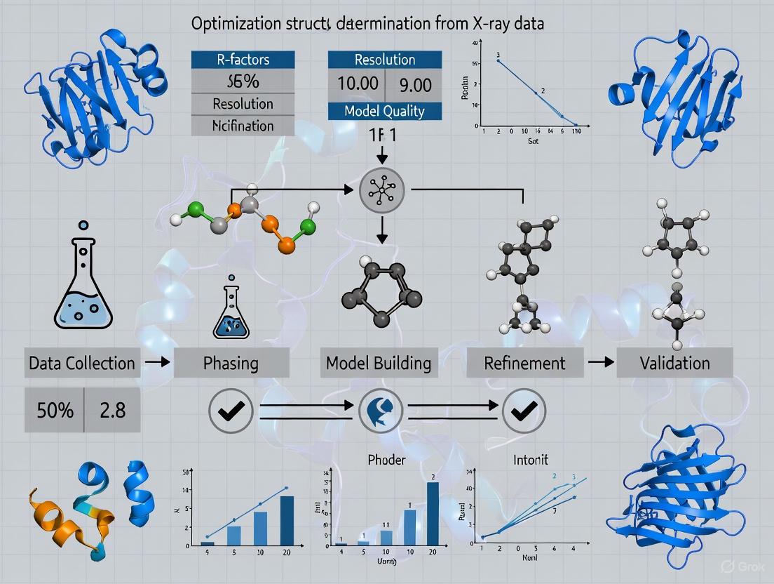
The complete process of determining a protein structure via X-ray crystallography follows a multi-stage workflow, from protein production to final model validation and deposition.
Figure 1: Comprehensive workflow for protein structure determination by X-ray crystallography. Key optimization points (yellow) include crystallization, phase determination, and model building.
Protein Crystallization Protocols
Initial Crystal Screening
Purpose: To identify initial conditions that promote protein crystallization using sparse matrix screens.
Materials:
- Purified, concentrated protein (>10 mg/mL in low-salt buffer)
- 96-well crystallization screening kits (commercial or custom)
- Crystallization plates (sitting-drop or hanging-drop vapor diffusion)
- Sealing tapes or oils
- Automated liquid handling system (e.g., mosquito Xtal3) [5]
Procedure:
- Plate Preparation: Label crystallization plates and add reservoir solutions (50-100 μL) to each well using an automated dispenser or multichannel pipette.
- Drop Setup: For each condition, mix:
- 100-200 nL protein solution
- 100-200 nL reservoir solution Use crystallization robots like the mosquito Xtal3 for precise nanoliter-scale dispensing [5].
- Sealing: Seal plates with transparent tape to prevent evaporation.
- Incubation: Incubate plates at constant temperature (4°C, 20°C, or 37°C) without disturbance.
- Monitoring: Check plates regularly under a microscope for crystal formation (days to weeks).
Crystal Optimization
Purpose: To refine initial crystallization hits to produce larger, well-ordered crystals.
Materials:
- Optimized crystallization screens (customized using systems like dragonfly with MXone mixer) [5]
- Additive screens
- Microseeding tools
Procedure:
- Grid Screening: Set up fine-scale screens around initial hit conditions, varying:
- Precipitant concentration (±10-40% of original)
- pH (±0.2-0.5 units)
- Temperature (4°C, 20°C, 37°C)
- Additive Screening: Include additives (0.1-5% concentration) such as salts, detergents, or small molecules.
- Seeding: Transfer microcrystals from initial hits to new drops to promote growth.
- Evaluation: Assess crystal quality by size, morphology, and ultimately by X-ray diffraction.
Data Collection Strategies
Crystal Cryoprotection and Mounting
Purpose: To preserve crystal structure during data collection by preventing ice formation and radiation damage.
Materials:
- Cryoprotectant solutions (e.g., glycerol, ethylene glycol, sucrose)
- Cryo-loops of appropriate sizes
- Liquid nitrogen storage Dewars
- Synchrotron beamline or in-house X-ray source
Procedure:
- Cryoprotectant Testing: Test cryoprotectant solutions by adding them to reservoir solution at increasing concentrations (5-25%).
- Soaking: Soak crystals in final cryoprotectant solution for 5-30 seconds.
- Mounting: Mount crystal in cryo-loop and flash-cool in liquid nitrogen stream.
- Storage: Transfer to liquid nitrogen Dewar for storage or shipping to synchrotron.
X-ray Data Collection
Purpose: To collect complete, high-quality diffraction data.
Materials:
- Synchrotron beamline with robotic sample changer
- X-ray detector
- Goniometer for crystal positioning
Procedure:
- Screening: Collect preliminary diffraction images to assess crystal quality.
- Strategy Calculation: Use beamline software to determine optimal data collection strategy.
- Data Collection: Collect complete dataset by rotating crystal through appropriate angular range with optimal exposure time.
- Assessment: Monitor data quality metrics (resolution, completeness, signal-to-noise) during collection.
Modern Serial Crystallography Methods
Serial crystallography (SX) has revolutionized structural biology by enabling high-resolution structure determination from microcrystals, studying reaction mechanisms, and expanding the range of biomolecules amenable to structural analysis [1]. This approach is particularly valuable for proteins that only form small crystals or for time-resolved studies.
Table 2: Sample Delivery Methods in Serial Crystallography
| Method | Principle | Sample Consumption | Optimal Applications |
|---|---|---|---|
| Fixed-Target | Crystals are arrayed on a solid support and scanned through X-ray beam | Very low (nanograms) | Precious samples, high-throughput screening |
| Liquid Injection | Crystal slurry is continuously injected as a liquid jet | High (milligrams) | Abundant samples, time-resolved studies |
| High-Viscosity Extrusion | Crystals are embedded in viscous matrix and extruded | Medium (micrograms) | Reduced flow rate, lower sample consumption |
| Hybrid Methods | Combination of fixed support with flow capabilities | Variable | Flexible experimental designs |
The theoretical minimum sample requirement for a complete SX dataset is approximately 450 ng of protein, assuming microcrystal dimensions of 4×4×4 μm, protein concentration of 700 mg/mL in the crystal, and 10,000 indexed patterns [1]. Recent advances have dramatically reduced sample consumption from gram quantities in early experiments to microgram amounts today [1].
Structure Solution and Refinement
Phase Determination Protocols
Molecular Replacement
Purpose: To determine initial phases using a known homologous structure.
Materials:
- Homologous search model (from PDB or AlphaFold prediction)
- Molecular replacement software (PHASER, MOLREP)
- Processed diffraction data (amplitudes |F|)
Procedure:
- Model Preparation: Edit search model to match target sequence and remove non-conserved regions.
- Rotation Function: Search for correct orientation of model in unit cell.
- Translation Function: Determine position of correctly oriented model.
- Phase Calculation: Generate initial phases from positioned model.
- Model Building: Use experimental density to correct and rebuild model.
Experimental Phasing (SAD/MAD)
Purpose: To determine phases experimentally using anomalous scatterers.
Materials:
- Derivative crystals with incorporated heavy atoms
- Single- or multi-wavelength diffraction data
- Experimental phasing software (AutoSol, SHARP)
Procedure:
- Heavy Atom Derivatization: Soak crystals in heavy atom solutions or incorporate selenomethionine.
- Data Collection: Collect single-wavelength (SAD) or multi-wavelength (MAD) data.
- Substructure Solution: Locate heavy atom positions in unit cell.
- Phase Calculation: Calculate experimental phases from anomalous differences.
- Density Modification: Improve phases through solvent flattening and histogram matching.
Advanced Computational Integration
Recent advances in machine learning have transformed structural biology, enabling new approaches to structure determination. The ROCKET method augments AlphaFold2 by refining its predictions using experimental data from cryo-EM, cryo-ET, and X-ray crystallography [4]. This approach captures biologically important structural variation that AlphaFold2 alone does not, automating difficult modeling tasks such as flips of functional loops and domain rearrangements [4].
For low-resolution data, the XDXD framework represents a breakthrough as the first end-to-end deep learning approach to determine a complete atomic model directly from low-resolution single-crystal X-ray diffraction data [3]. This diffusion-based generative model bypasses the need for manual map interpretation, producing chemically plausible crystal structures conditioned on the diffraction pattern [3]. On a benchmark of 24,000 experimental structures, XDXD achieved a 70.4% match rate for structures with data limited to 2.0 Å resolution, with a root-mean-square error (RMSE) below 0.05 [3].
Optimization Techniques and Advanced Applications
Temperature Considerations in Data Collection
While more than 90% of protein crystal structures in the PDB were determined at cryogenic temperatures (100 K), growing awareness of potential artifacts and loss of physiologically relevant information has driven increased interest in data collection at room temperature or body temperature (37°C) [6]. Temperature significantly influences atomic motions and protein flexibility, which play crucial roles in enzymatic catalysis and allosteric communications [6].
Protocol for Temperature-Dependent Studies:
Purpose: To investigate temperature effects on protein structure and metal binding.
Materials:
- Temperature-controlled crystallography systems
- Dehydration prevention devices
- Reduced exposure data collection strategies
Procedure:
- Crystal Stability: Test crystal stability at target temperature prior to data collection.
- Radiation Damage Mitigation: Collect data with attenuated beam and multiple crystal positions.
- Hydration Maintenance: Ensure crystal remains hydrated throughout data collection.
- Rapid Data Collection: Use modern fast detectors to complete data collection before significant radiation damage occurs.
Studies of metal-protein adducts at body temperature have revealed that temperature can affect both protein conformation and metal coordination geometry, providing more physiologically relevant structural information [6]. For example, research on hen egg white lysozyme (HEWL) adducts with rhenium compounds showed that while Re binding sites were retained at 37°C with minor modifications, lower occupancy or absence of Re-containing fragments was observed in non-covalent binding sites compared to cryogenic structures [6].
The Scientist's Toolkit: Essential Research Reagents and Materials
Table 3: Essential Research Reagents and Materials for Protein Crystallography
| Reagent/Material | Function | Application Notes |
|---|---|---|
| Crystallization Screening Kits | Identify initial crystallization conditions | Commercial sparse matrix screens cover diverse chemical space |
| Cryoprotectants (glycerol, PEG) | Prevent ice formation during cryocooling | Must be optimized for each crystal type to avoid damage |
| Heavy Atom Compounds | Experimental phasing via anomalous scattering | Soaking concentrations and times require optimization |
| Ligands/Substrates | Study protein-ligand interactions | Co-crystallization or soaking approaches possible |
| Crystallization Robots | Automated nanoliter-scale setup | mosquito Xtal3 enables 30-50 nL drops for screening [5] |
| Liquid Handling Systems | Custom screen preparation | dragonfly with MXone mixer enables rapid optimization [5] |
| Synchrotron Beam Access | High-intensity X-ray source | Essential for weakly diffracting crystals and time-resolved studies |
| Cryo-EM for Small Proteins | Structure determination when crystallization fails | Coiled-coil fusion strategy enables study of small proteins like kRasG12C [7] |
Data Validation and Quality Assessment
The final step in any crystallographic structure determination is rigorous validation of the structural model. Key quality metrics include the R-factor and R-free, which assess how well the model explains the experimental data, with lower values indicating better agreement [2]. Additionally, validation tools assess stereochemical parameters (bond lengths, angles, torsion angles) and compare them to expected values from high-quality structures [2].
The resulting structural model, along with the experimental data and metadata, is typically deposited in the Protein Data Bank (PDB), which runs its own validation before releasing the structure to the public [2]. When selecting structures from the PDB for research applications, it is essential to assess validation reports and consider resolution, R-factors, and geometric quality to ensure the structural model is appropriate for the intended use [2].
Serial crystallography (SX) represents a paradigm shift in macromolecular structure determination, emerging initially at X-ray free-electron lasers (XFELs) and later adapted to synchrotron sources. This approach distributes radiation damage across thousands of microcrystals, enabling room-temperature data collection that captures protein structures in near-physiological states with minimal radiation damage. Serial Femtosecond Crystallography (SFX) utilizes ultrafast XFEL pulses that outrun most radiation damage processes through the "diffraction-before-destruction" principle, making it ideal for studying irreversible reactions and radiation-sensitive systems. Serial Millisecond Crystallography (SMX) adapts this methodology to synchrotron radiation sources, where exposure times are necessarily longer but beam access is more readily available. The development of high-viscosity injectors, particularly those using lipidic cubic phase (LCP), has dramatically reduced sample consumption from gram quantities to milligram or even microgram levels, opening these techniques to a broader range of biological targets, including challenging membrane proteins [8] [1] [9].
Table: Fundamental Characteristics of SFX and SMX
| Feature | SFX (X-FEL) | SMX (Synchrotron) |
|---|---|---|
| X-ray Source | X-ray Free-Electron Laser (XFEL) | Synchrotron storage ring |
| Pulse Duration | Femtoseconds (∼40-75 fs) [9] | Milliseconds (10-50 ms) [10] |
| Key Principle | "Diffraction-before-destruction" [9] | Dose distribution across many crystals [8] |
| Primary Advantage | Outrunning radiation damage; ultrafast time-resolved studies [9] | Wider accessibility; high room-temperature data quality comparable to cryo-data [8] |
| Typical Sample Consumption | ~100 μg - 1 mg per dataset [9] | <1 mg per dataset [8] |
| Data Collection Rate | 30 - 120 Hz [9] | 10 - 50 Hz [8] |
Comparative Performance and Applications
The implementation of SFX and SMX has enabled new scientific inquiries across structural biology. SFX provides unique capabilities for time-resolved studies on femtosecond to millisecond timescales, allowing researchers to capture molecular movies of reaction intermediates. SMX, while not as fast, offers a more accessible route for determining high-quality room-temperature structures of radiation-sensitive proteins and complexes. Room-temperature structures often reveal enhanced conformational flexibility and more biologically realistic ligand-binding states compared to traditional cryo-cooled structures, as freezing can trap non-equilibrium conformations [8] [9].
Table: Representative Experimental Outcomes from SFX and SMX
| Protein Target | Technique | Resolution (Å) | Key Experimental Details | Reference |
|---|---|---|---|---|
| Bacteriorhodopsin (bR) | SFX (LCP injector) | 2.3 | Time-resolved study with 1 ms delay; sample consumption ~1 mg/time point [9] | Weierstall et al., 2014 |
| Bacteriorhodopsin (bR) | SMX (LCP injector) | 2.4 | Room-temperature structure; similar to SFX but with distinct retinal pathway details [10] | Nogly et al., 2015 |
| Mo Storage Protein (MOSTO) | SMX | ~1.8 | High-resolution structure of radiation-sensitive protein [8] | Botha et al., 2017 |
| A2A Adenosine Receptor | SMX | ~2.2 | Native sulfur-SAD phasing demonstrated [8] | Botha et al., 2017 |
| Tubulin-Darpin Complex | SMX | ~2.1 | Successful soaking of drug colchicine demonstrated [8] | Botha et al., 2017 |
SMX Experimental Protocol: LCP-Based Sample Delivery
Materials and Equipment
- Purified Protein: 9-15 mg/mL in appropriate detergent (e.g., 1.2% β-OG for bacteriorhodopsin) [10]
- Monoolein: Lipid for forming lipidic cubic phase [10]
- Precipitant Solution: e.g., 29-38% PEG 2000, 100 mM phosphate buffer pH 5.6 [10]
- Syringe Coupler: For mixing protein and lipid [10]
- High-Viscosity Injector: LCP injector with 20-75 μm diameter nozzles [8] [9]
- Synchrotron Microfocus Beamline: Equipped with high-frame-rate detector (e.g., EIGER 16M) [8]
Step-by-Step Procedure
1. Crystallization in LCP:
- Mix purified protein with monoolein in a 40:60 (v/v) ratio using syringe coupler [10].
- Extrude mixture repeatedly (20-30 passes) to form homogeneous LCP.
- Load LCP into 100 μL syringe and overlay with precipitant solution.
- Incubate at 20°C in the dark until microcrystals form (typically several days) [10].
2. Sample Preparation for Injection:
- Remove excess precipitant solution from crystallization syringe.
- Add pure monoolein to adjust crystal density.
- Homogenize crystal-LCP mixture using syringe coupler to break larger crystals into fragments <50 μm [10].
- Load homogenized sample into LCP injector.
3. Data Collection:
- Align LCP stream (extruded at 50-250 nL/min) with microfocus X-ray beam (e.g., 20 × 5 μm) [8].
- Collect diffraction patterns with 10-50 ms exposure per pattern at 50 Hz frame rate.
- Continue data collection until ~10,000-100,000 patterns are acquired (typically 1-20 hours) [8].
4. Data Processing:
- Index and integrate diffraction patterns using software such as CrystFEL.
- Merge data from all crystals to create complete dataset.
- Solve structure by molecular replacement or de novo phasing.
- Refine structure using standard crystallographic software [8] [10].
SFX Experimental Protocol: Time-Resolved Studies
Materials and Equipment
- Microcrystals: 10-15 μm size for uniform light penetration [9]
- High-Viscosity Injector: LCP injector with 20-50 μm diameter nozzles [9]
- Optical Pump Laser: Femtosecond laser synchronized with XFEL pulses [9]
- XFEL Source: e.g., Linac Coherent Light Source (LCLS) [9]
Step-by-Step Procedure
1. Sample Preparation:
- Prepare concentrated microcrystals in LCP as described in SMX protocol.
- Optimize crystal density for hit rates of 5-10% at XFEL repetition rate.
- Load sample into LCP injector.
2. Experimental Setup:
- Align LCP stream with XFEL beam (typically 1.5 × 1.5 μm focus).
- Synchronize optical pump laser with XFEL pulses at desired repetition rate (e.g., 30 Hz pumping with 120 Hz XFEL) [9].
- Set desired time delay between pump and probe pulses.
3. Data Collection:
- Collect single diffraction pattern from each crystal intercepted by XFEL pulse.
- Attenuate X-ray pulses to prevent detector damage while maintaining sufficient signal.
- Acquire 10,000-100,000 indexed patterns per time delay.
4. Data Processing:
- Process data similarly to SMX but account for specific XFEL properties.
- Calculate difference Fourier maps between light-activated and dark states.
- Refine structures for each time delay to reconstruct reaction trajectory [9].
Workflow Visualization
Serial Crystallography Workflow Selection
Research Reagent Solutions
Table: Essential Materials for Serial Crystallography
| Reagent/Equipment | Function/Application | Technical Specifications |
|---|---|---|
| Lipidic Cubic Phase (LCP) | Viscous delivery medium for membrane proteins and microcrystals [9] [10] | Monoolein lipid; protein:lipid ratio ~40:60 (v/v); low extrusion rate (50-250 nL/min) |
| High-Viscosity Injector | Extrudes crystal-laden medium into X-ray beam [8] [9] | Nozzle diameter: 20-75 μm; flow rate: 0.05-2 μL/min; compatible with viscous media |
| High-Frame-Rate Detector | Records diffraction patterns at high repetition rates [8] | EIGER 16M; frame rates: 50-120 Hz; high dynamic range |
| Microfocus Beamline | Provides intense, focused X-ray beam for SMX [8] [10] | Beam size: 5×5 to 20×5 μm²; flux: 10¹¹-10¹² ph/s; compatible with injector setups |
| XFEL Source | Provides ultrafast, high-intensity pulses for SFX [9] | Pulse duration: ~75 fs; repetition rate: 30-120 Hz; high peak brightness |
Serial crystallography (SX), conducted at both synchrotrons and X-ray free-electron lasers (XFELs), has revolutionized structural biology by enabling high-resolution structure determination at room temperature with minimal radiation damage [1]. This technique relies on collecting diffraction patterns from thousands of microcrystals, each exposed to an X-ray pulse only once, following the "diffraction before destruction" principle [11]. The efficiency of these experiments is fundamentally constrained by the effective delivery of precious crystal samples to the X-ray interaction point. Sample consumption remains a critical challenge, as the limited availability of many biologically significant macromolecules makes efficient use of purified protein essential [1] [12]. Innovations in sample delivery methodologies—primarily categorized as fixed-target, liquid injection, and hybrid systems—are therefore pivotal for optimizing protein structure determination workflows. These systems aim to maximize the crystal hit rate while minimizing sample waste, thereby expanding the range of accessible biological targets, including complex membrane proteins and dynamic enzymatic complexes studied via time-resolved methods [13] [14].
Comparative Analysis of Sample Delivery Methods
The performance of different sample delivery systems can be evaluated based on key parameters such as sample consumption, hit rate, compatibility with time-resolved studies, and operational complexity. The following sections and tables provide a detailed comparison to guide researchers in selecting the appropriate method for their experimental needs.
Table 1: Key Characteristics of Major Sample Delivery Methods
| Method | Typical Sample Consumption | Relative Hit Rate | Compatibility with Time-Resolved Studies | Key Advantages | Major Limitations |
|---|---|---|---|---|---|
| Liquid Injection (GDVN) | ~10 mg to 1 g [1] [11] | Medium | High (Excellent for mix-and-inject) [1] | Maintains crystal hydration; continuous flow [11] | High sample waste at low repetition rates; shear forces on crystals [11] [13] |
| High-Viscosity Extrusion | ~1-10 mg [11] [13] | High | Medium (Compatible with LCP-grown crystals) [11] | Reduced flow rates; protects sensitive crystals [13] | Potential interactions between matrix and sample [13] |
| Fixed-Target Scanning | <1 mg [1] [15] | High | High (Excellent for pump-probe) [15] [14] | Minimal sample waste; precise crystal positioning [16] [14] | Risk of crystal drying; requires synchronization [15] |
| Droplet-Based Hybrid | Microgram quantities [1] | Medium to High | High [17] | Dramatically reduced sample waste [17] | Requires complex synchronization with X-ray pulses [17] |
Table 2: Theoretical Minimum Sample Requirement for a Complete Dataset
| Parameter | Theoretical Value | Description |
|---|---|---|
| Indexed Patterns Required | 10,000 | Typical number for a full dataset [1] |
| Assumed Crystal Size | 4 × 4 × 4 µm | Example microcrystal dimension [1] |
| Protein Concentration in Crystal | ~700 mg/mL | Based on a 31 kDa protein (e.g., NQO1) [1] |
| Theoretical Minimum Protein Mass | ~450 ng | Calculated ideal minimum consumption [1] |
Detailed Methodologies and Application Notes
Fixed-Target Systems
Fixed-target methods involve mounting microcrystals onto a solid, stationary support that is then scanned through the X-ray beam [15] [14]. This approach is renowned for its high sample efficiency.
Protocol: Data Collection Using a Cyclic Olefin Copolymer (COC) Fixed-Target Device
Key Research Reagent Solutions:
- COC Fixed-Target Chip: Fabricated with up to 18,000 crystal traps, each designed to hold a single crystal up to 50 µm in size. The COC material provides low X-ray background scattering [16].
- Crystal Slurry: A concentrated suspension of microcrystals in their mother liquor or a suitable stabilizing solution.
- Humidity Chamber: To prevent dehydration of crystals during loading and data collection.
Procedure:
- Sample Loading: Apply 1-2 µL of crystal slurry directly onto the surface of the COC chip. Use a gentle air stream or a wicking tool to remove excess mother liquor, ensuring crystals are seated within the traps [16].
- Chip Mounting: Secure the loaded chip into the sample holder of the fixed-target sample chamber (e.g., the FT-SFX chamber at PAL-XFEL) [15].
- Alignment: Align the chip relative to the X-ray beam path using the chamber's translation stages and real-time microscopy monitoring.
- Data Collection Scripting: Program a raster scanning pattern. The scan parameters (step size, speed) should be optimized to match the XFEL repetition rate (e.g., 60 Hz at PAL-XFEL) and ensure no crystal is hit twice [15].
- Data Collection: Initiate the scanning sequence and X-ray exposure. For weak diffraction signals, conduct the experiment in a helium-purged environment to minimize air scattering [15].
Workflow Diagram
Fixed-Target Experimental Workflow
Liquid Injection Systems
Liquid injectors continuously deliver a stream of crystal suspension into the X-ray beam. A major innovation in this category is the Gas Dynamic Virtual Nozzle (GDVN), which uses a co-flowing gas to focus a liquid jet down to micrometer diameters, preventing clogging [11].
Protocol: SFX using a GDVN Injector at an XFEL
Key Research Reagent Solutions:
- GDVN Nozzle: Consists of a tapered liquid capillary (e.g., 50 µm inner diameter) surrounded by a coaxial gas capillary. The helium gas flow focuses the liquid jet to diameters as small as 4 µm [11] [13].
- High-Pressure HPLC Pump: Delivers the crystal suspension at a stable, pressurized flow.
- Crystal Suspension: A homogeneous slurry of microcrystals at a high concentration (e.g., 10⁹ to 10¹⁰ crystals/mL) [11].
Procedure:
- Nozzle Preparation: Assemble the GDVN nozzle ensuring the liquid and gas capillaries are clean and aligned.
- Sample Loading: Load the crystal suspension into the sample reservoir, taking care to avoid sedimentation.
- Injector Alignment: Install the nozzle into the injection chamber (e.g., the MICOSS system at PAL-XFEL) and align the jet to intersect the X-ray beam using in-line cameras [13].
- Flow Initiation: Start the liquid flow and adjust the liquid pressure (typically to achieve ~10 µL/min) and gas pressure to establish a stable, unbroken jet.
- Data Collection: Trigger the X-ray pulses and detector to record diffraction patterns from crystals randomly oriented in the jet. A full dataset often requires several hours of continuous operation and 10-100 mL of sample suspension [11].
To address the high sample waste of continuous jets, high-viscosity injectors have been developed. These extrude crystals embedded in a media like lipidic cubic phase (LCP) or other viscous matrices at flow rates as low as 300 nL/min, drastically reducing consumption [11] [13].
Hybrid Delivery Systems
Hybrid systems combine features of both injector and fixed-target methods to leverage their respective advantages. A prominent example is the droplet-on-demand system, which generates segmented crystal-laden droplets separated by an immiscible oil [17].
Protocol: Droplet-Based Sample Delivery for Reduced Waste
Key Research Reagent Solutions:
- 3D-Printed Microfluidic Chip: Integrates droplet generation and nozzle injection in a single device. Contains channels for sample and immiscible oil.
- Immiscible Oil Phase: A biocompatible oil (e.g., perfluorinated oil) that acts as a spacer between aqueous sample droplets.
- Precision Syringe Pumps: To control the flow rates of both the sample and oil phases.
- Electrical Triggering System: For synchronizing droplet generation with XFEL pulses [17].
Procedure:
- Device Priming: Prime the microfluidic channels with the immiscible oil to ensure stable droplet formation.
- Droplet Generation: Initiate flow of both the crystal suspension and the oil. The device geometry generates monodisperse aqueous droplets within the oil stream.
- Synchronization: Use the electrical triggering system to synchronize the release of droplets so that a fresh droplet arrives at the X-ray interaction point for each XFEL pulse. This ensures that sample between pulses is oil, not precious crystal suspension [17].
- Injection and Data Collection: The droplet stream is injected into the chamber towards the X-ray beam. Diffraction data is collected only when a droplet is in the beam path.
Workflow Diagram
Hybrid Droplet-Based Experimental Workflow
Integrated System for Time-Resolved Studies
Fixed-target and hybrid systems are particularly advantageous for time-resolved serial crystallography (TR-SX), which aims to capture molecular movies of biochemical reactions [1] [14]. Fixed-target chips allow for precise reaction initiation on the chip itself, either by light (pump-probe) or by rapid mixing of substrates with crystals, followed by scanning at defined time delays [14]. The consistency in sample preparation and delivery between synchrotron (SSX) and XFEL (SFX) sources when using fixed targets allows for direct comparison of structures across time scales and facilities, validating observed conformational changes [14].
The ongoing innovation in sample delivery systems is a cornerstone of modern protein structure determination. Fixed-target, liquid injection, and hybrid methods each offer distinct profiles of sample efficiency, operational complexity, and applicability to dynamic studies. The choice of system must be tailored to the specific protein target, the scientific question—particularly for time-resolved experiments—and the available beamline infrastructure. As these technologies continue to mature, converging towards the theoretical minimum of sample consumption, they will unlock unprecedented opportunities for determining the structures of previously intractable biological macromolecules and visualizing their functional dynamics in real time.
The field of structural biology is undergoing a profound transformation, driven by the ability to generate data at an unprecedented scale. The advent of high-throughput techniques, particularly in crystallographic fragment screening, is revolutionizing drug discovery but simultaneously precipitating a data management crisis. With specialized synchrotron facilities capable of conducting over 150 fragment-screening campaigns annually—a number poised to exceed 1,000 as global facilities reach full capacity—the research community faces the challenge of managing an estimated one million individual diffraction datasets and up to 100,000 new protein-ligand structures each year [18]. This deluge of data, often reaching terabyte scales per campaign, necessitates a fundamental re-evaluation of traditional data processing, storage, and archival practices. This application note details the current landscape, quantitative challenges, and essential protocols for managing terabyte-scale crystallography datasets within the broader context of optimizing protein structure determination workflows.
The Quantitative Scale of the Data Challenge
The transition to high-throughput methods has fundamentally altered the data volume in crystallography. The table below quantifies key aspects of this data revolution, highlighting the immense scale and its implications for data management.
Table 1: Quantitative Overview of High-Throughput Crystallography Data Generation
| Aspect | Traditional Crystallography | High-Throughput Fragment Screening | Data Management Implication |
|---|---|---|---|
| Campaigns/Year | Dozens | >150 (currently), ~1,000 (projected at capacity) [18] | Linear scaling of raw data and results requiring storage |
| Datasets/Campaign | 1 - 10 | ~1,000 compounds [18] | Millions of datasets annually across all facilities |
| Structures/Year | ~10,000 new crystal structures in PDB [18] | ~100,000 additional protein-ligand structures [18] | Overwhelms traditional deposition and curation pipelines |
| Data Arrival Rate | Hours to days | Seconds after collection at detector [19] | Requires real-time streaming and processing infrastructure |
| Representative Data Volume | Gigabytes (GB) | Terabytes (TB) to hundreds of TB [19] | Demands scalable, high-performance storage architectures |
This exponential growth is not limited to fragment screening. Other applications, such as the masked autoencoder for X-ray image encoding (MAXIE), are trained on datasets as large as 286 terabytes of X-ray diffraction images [19]. Furthermore, at facilities like the Linac Coherent Light Source (LCLS-II), X-ray laser shot repetition rates have increased to 1 MHz, generating electron time-of-flight data with sub-femtosecond resolution and creating immense data streams that require online analysis for experimental steering [19].
Experimental Protocols for High-Throughput Data Management
Protocol: Implementing an End-to-End Data Streaming Framework
Coupling high-performance computing (HPC) resources with external, online data sources is critical for real-time analysis. The LCLStream ecosystem provides a proven framework for this purpose [19].
- Objective: To enable real-time streaming of experimental data from detectors to remote HPC resources for immediate processing and analysis.
- Materials:
- LCLStream API Server or equivalent middleware.
- High-rate data buffer (e.g., NNG-Stream).
- Mutual authentication framework (certificate-driven).
- HPC cluster with access to data processing libraries (e.g., psana2).
- Procedure:
- Data Request: An external user or beamline system requests a specific dataset from an active experiment using a REST API with a JSON-formatted query [19].
- Mutual Authentication: The user and server authenticate each other using digital certificates to ensure security [19].
- Job Launch: The API server creates a unique JobID and launches the
LCLStreamerandNNG-Streamcomponents on the local computing cluster (e.g., SLAC's S3DF cluster) [19]. - Data Reduction & Streaming: The
LCLStreamerapplication reads event data using facility-specific libraries (e.g., psana2), performs user-defined partial data reduction, and formats the output. - Buffered Transfer: The
NNG-Streamcomponent buffers data between parallel producers and consumers, smoothing network bursts and enabling traversal of complex network topologies [19]. - Data Consumption: Processed data is delivered to external applications, which can include supercomputer centers for AI training, network appliances, or automated control systems for experimental feedback [19].
- Outcome: Preliminary results show data can arrive at a remote HPC job, such as one at Oak Ridge National Laboratory, just seconds after collection at detectors in Menlo Park, enabling near-real-time analysis [19].
Protocol: Architectural Design for Scalable Data Management
Proper data management must be considered from the first day of setting up an imaging or crystallography lab to avoid costly data recovery and organizational problems later [20].
- Objective: To establish a scalable and accessible data management architecture for large, heterogeneous crystallography datasets.
- Materials:
- Managed web-browser interface (e.g., DigiM I2S or similar).
- Relational database for metadata indexing.
- Scalable storage solution (cloud, NAS, or server).
- Computational resources for automated processing.
- Procedure:
- Automated Cataloguing: Implement a system that automatically generates visual thumbnails of datasets upon ingestion, creating a searchable visual catalogue [20].
- Metadata Capture: Record all experimental metadata (e.g., date stamps, user, sample information, beamline parameters) concurrently with data acquisition into a relational database [20].
- Workflow Integration: Conduct data analysis within the managed environment so that all processing steps, parameters used, and derived data are automatically recorded and annotated [20].
- Queue Management: Utilize a job queuing system that allows users to submit long computational tasks and receive email notifications with hyperlinks to results upon completion [20].
- Universal Indexing and Search: Ensure that every piece of data, metadata, and analysis result is indexed and made searchable through the browser interface, moving beyond simple file explorer capabilities [20].
- Plan for Scaling: Adopt a nested client-server architecture that abstracts user access, computing, and storage needs through API layers, allowing the system to scale from dozens to thousands of datasets and users [20].
The following diagram illustrates the logical flow and components of this managed architecture.
Data Management Architecture: Logical workflow for a scalable system that integrates data storage, metadata indexing, and computational processing.
Computational Workflows for Automated Structure Determination
The volume of data generated by high-throughput crystallography makes manual processing impossible. Automated software pipelines are essential.
Table 2: Key Software Tools for High-Throughput Data Processing
| Software Tool | Primary Function | Key Feature | Application Context |
|---|---|---|---|
| AutoPD [21] | Automated meta-pipeline | Integrates AlphaFold-assisted molecular replacement and adaptive decision-making | High-throughput structure determination from raw data to model |
| APEX Suite [22] | Instrument control to publication | AI-based crystal centering and STRUCTURE NOW plugin for automated solution | Laboratory (in-house) single-crystal X-ray diffraction |
| PanDDA [18] | Hit-finding from fragment screens | Pan-Dataset Density Analysis to identify low-occupancy binders | High-throughput crystallographic fragment screening |
| DIALS [23] | Data integration | Modern package designed for data from synchrotrons and XFELs | Processing challenging datasets from modern sources |
| LCLStreamer [19] | Data streaming & reduction | Flexible API-driven data requests and real-time streaming to HPC | On-line data analysis and experimental steering at large facilities |
Protocol: Automated Structure Determination with AutoPD
AutoPD is an open-source meta-pipeline designed to address the automation challenge from raw data to high-precision structural models [21].
- Objective: To automatically determine a protein structure from raw diffraction data and an amino acid sequence file.
- Materials:
- Raw diffraction images (e.g., in HDF5 or SMV format).
- Protein amino acid sequence file (FASTA format).
- Access to a high-performance computing cluster.
- AutoPD software installation.
- Procedure:
- Data Ingestion and Integration: AutoPD ingests the raw diffraction images and performs initial data reduction (indexing, integration, and scaling) using integrated processing engines [21].
- Adaptive Decision-Making: The pipeline dynamically selects the optimal structure modeling pathway based on data quality and intermediate results [21].
- Structure Solution:
- Model Building and Refinement: The pipeline performs iterative cycles of automated model building and refinement.
- Validation and Output: The final model and electron density maps are generated and validated. The pipeline achieves a success rate of 92% on benchmark datasets, with map-model correlation values of at least 0.5 [21].
The workflow of this automated pipeline, highlighting its adaptive decision points, is shown below.
AutoPD Workflow: Automated pipeline for protein structure determination that adaptively chooses the best solution path.
The Scientist's Toolkit: Research Reagent Solutions
Successful navigation of the data revolution requires both cutting-edge software and robust physical materials. The following table details essential reagents and materials for high-throughput crystallography workflows, with a focus on membrane proteins as a challenging and biologically relevant case study [24].
Table 3: Essential Research Reagents for High-Throughput Crystallography
| Reagent / Material | Function / Purpose | Example Types / Notes |
|---|---|---|
| Expression Vectors | Cloning and expressing the target protein; tags aid purification. | pET20b, pET-DUET, pRSF-1b; often modified with N-terminal pelB signal sequence and His-tags [24]. |
| Host Cell Lines | Protein expression system; different lines address toxicity and codon usage. | BL21(DE3) for standard expression; C41/C43 for toxic genes; Rosetta for rare codons [24]. |
| Detergents | Solubilizing and stabilizing membrane proteins post-cell lysis. | DDM, LDAO, OG, C8E4, LMNG; must be kept above critical micelle concentration (CMC) [24]. |
| Affinity Chromatography Resins | Primary purification step to isolate the target protein from cell lysate. | Ni-NTA resin for His-tagged proteins; Strep-Tactin resin for Strep-tagged proteins [24]. |
| Crystallization Screens | Initial screening of conditions to nucleate protein crystals. | Commercial screens specifically marketed for membrane proteins (e.g., MemGold, MemSys) [24]. |
| Lipid/Additive Supplements | Enhancing protein stability and promoting crystallization. | Cholesterol, specific lipids; used as additives in purification or crystallization buffers [24]. |
| Rare-Earth Doped Crystals | Potential future medium for high-density data storage. | Praseodymium-doped Yttrium oxide; uses crystal defects for atomic-scale memory cells [25] [26]. |
The data revolution in crystallography is an undeniable reality. The paradigms of manual data handling and processing are no longer viable in an era of terabyte-scale campaigns. The future of efficient protein structure determination hinges on the widespread adoption of the integrated strategies outlined in this note: real-time data streaming frameworks, scalable and managed data architectures, and highly automated computational pipelines. Furthermore, the community must collectively address the impending challenge of data archival, as current procedures for deposition into the Protein Data Bank are not designed for the influx of hundreds of thousands of structures annually from fragment screens alone [18]. Embracing this revolution by implementing robust data management protocols is no longer optional but a fundamental requirement for continued success in structural biology and structure-based drug discovery.
Current Market and Technology Landscape for Protein Crystallography
The global protein crystallography market is experiencing robust growth, propelled by its indispensable role in structural biology and rational drug design. By creating ordered, structured lattices for complex macromolecules, this technique enables high-resolution structure determination that is crucial for understanding biological function and developing targeted therapeutics [27]. The market's expansion is fundamentally driven by increasing demand for protein-based therapeutics, rising investments in biopharmaceutical research and development (R&D), and continuous technological advancements that enhance experimental throughput and success rates [27] [28].
Table 1: Global Protein Crystallography Market Size and Growth Projections
| Market Size Year | Market Value (USD Billion) | Projected Year | Projected Value (USD Billion) | Compound Annual Growth Rate (CAGR) | Source |
|---|---|---|---|---|---|
| 2024 | 1.62 | 2029 | 2.8 | 11.5% | [28] |
| 2024 | 6.80 | 2032 | 19.41 | 14.00% | [29] |
| 2025 | 1.82 | 2029 | 2.8 | 11.5% | [28] |
The growing adoption of biologics, including monoclonal antibodies and engineered enzymes, has created a sustained need for atomic-level structural data to support regulatory filings. Notably, the Protein Data Bank (PDB) has informed over 80% of antineoplastic approvals from 2019-2023, cementing structural evidence as a central component of drug dossiers [27]. Concurrently, substantial R&D investments from both public and private sectors are legitimizing capital expenditures on advanced crystallography platforms. Examples include the U.S. National Science Foundation's $40 million Use-Inspired Protein Design initiative and Thermo Fisher Scientific's $1.3 billion R&D expenditure in 2023, a substantive share of which was devoted to protein-analysis platforms [27].
Market Segmentation and Technological Trends
Analysis by Product, Technology, and End-User
The protein crystallography market can be segmented by product, technology, and end-user, each revealing distinct trends and growth trajectories.
Table 2: Market Segmentation and Key Characteristics (2024-2025)
| Segment | Category | Market Share or CAGR | Key Characteristics and Trends |
|---|---|---|---|
| By Product | Instruments | 44.23% of market size (2024) [27] | Includes X-ray diffractometers, liquid handlers, imaging systems. Purchasers prioritize photon-counting detectors and robotic samplers. |
| Software & Services | 12.19% CAGR [27] | Fastest-growing segment. Cloud-native suites enable remote collaboration and automated data processing. | |
| Reagents & Consumables | Mid-single-digit growth [27] | Steady demand for screens, kits, and cryoprotectants. Innovation in formulations, e.g., sodium-malonate. | |
| By Technology | X-ray Crystallography | 56.15% market share (2024) [27] | Dominant, well-established method. Ongoing detector upgrades tighten experimental cycle times. |
| Microfluidic Screening | 11.73% CAGR [27] | Offers dramatic sample volume reduction; crystal hits emerge in minutes, not days. | |
| Cryo-electron Microscopy (Cryo-EM) | Complementary growth [27] | Gaining traction for challenging samples but does not displace diffraction in regulatory settings. | |
| By End-User | Pharmaceutical & Biotech Companies | 54.22% market share (2024) [27] | Rely on internal beamlines for IP-sensitive targets; anchor commercial demand. |
| Contract Research Organizations (CROs) | 10.24% CAGR [27] | Highest growth due to outsourcing by smaller, cost-conscious firms. | |
| Academic & Research Institutes | Significant share [27] | Anchor basic methodological innovation; benefit from sustained government grants. |
Key Technological Trends Shaping the Field
Several transformative technological shifts are redefining protein crystallography workflows, making them more efficient, accessible, and powerful.
Automation and AI Integration: Crystallization robots with AI-powered screening capabilities are transforming the traditional trial-and-error paradigm into a data-driven process [29]. These systems can design, execute, and analyze hundreds of crystallization conditions in parallel, learning from previous outcomes to refine subsequent experiments. In data processing, cloud-native software suites offer automated phasing, model validation, and AI-assisted refinement, significantly accelerating the path from raw data to refined structure [27]. Tools like the AutoPD meta-pipeline demonstrate this trend, integrating AlphaFold-assisted molecular replacement and adaptive decision-making to automate structure determination from raw diffraction data [21].
Miniaturization and Microfluidics: High material cost and scarce protein samples have long throttled crystal growth, particularly for membrane proteins. Microfluidic chips address this challenge by reducing sample needs by an order of magnitude and screening thousands of conditions within minutes [27]. This miniaturization enables affordable fabrication, allowing mid-tier universities to adopt advanced workflows and broadening the technology's user base [27].
Advancements in Serial Crystallography (SX): Serial crystallography, conducted at X-ray free-electron lasers (XFELs) and synchrotrons, has revolutionized the field by enabling structure determination from micro- and nano-sized crystals at room temperature [1]. A primary focus of recent SX development has been on reducing sample consumption. While early SX experiments required grams of purified protein, advancements in sample delivery systems have shrunk this requirement to microgram amounts [1]. Efficient sample delivery methods, such as fixed-target systems and liquid injection, are critical for maximizing the potential of SX and expanding its application to a broader range of biologically significant samples [1].
Shift Towards Physiological Temperature Data Collection: There is a growing awareness that routine data collection at cryogenic temperatures (100 K) can introduce artifacts and obscure physiologically relevant conformational dynamics [6]. Consequently, more researchers are exploring data collection at room temperature or even body temperature (37°C) to capture functionally important protein flexibility and more accurate metal coordination geometries, which is particularly relevant for studying metallodrug interactions [6].
Regional Market Dynamics
The adoption and development of protein crystallography technologies vary significantly across geographic regions, influenced by local infrastructure, funding landscapes, and research priorities.
Table 3: Regional Market Analysis (2024)
| Region | Market Share / CAGR | Key Drivers and Infrastructure |
|---|---|---|
| North America | 36.13% of global revenue [27] | Supported by NIH and NSF programs; mature pharma clusters in Massachusetts and California; synchrotrons like APS and SSRL. |
| Asia-Pacific (APAC) | Fastest-growing region (10.05% CAGR through 2030) [27] | Rapidly growing investments in life sciences; China's next-generation synchrotron in Shanghai; government-incentivized public-private partnerships. |
| Europe | Significant share [27] | Coordinated EU investment (e.g., Diamond-II upgrade, European Spallation Source); regulatory harmonization facilitates cross-border research. |
Detailed Experimental Protocols
Protocol 1: Microcrystallization of Lysozyme for SFX
Lysozyme is a standard reference protein commonly utilized in initial Serial Femtosecond Crystallography (SFX) trials to optimize detector geometry and experimental setup [30]. This protocol details the production of ~5 µm microcrystals at 17°C.
Research Reagent Solutions
| Item | Function in the Protocol |
|---|---|
| Sodium Acetate Trihydrate | Component of the buffering system to maintain pH. |
| Acetic Acid | Component of the buffering system to maintain pH. |
| Sodium Chloride | Precipitant in the crystallization solution. |
| PEG 6000 (50% w/v) | Precipitant in the crystallization solution. |
| Lysozyme (Egg White) | The target protein for microcrystallization. |
| CellTrics Filter (30 µm) | To isolate microcrystals of the desired size. |
Materials and Equipment
- Sodium acetate trihydrate, Acetic acid, Sodium chloride, PEG 6000 (50% w/v), Lysozyme (egg white) [30]
- pH meter, Graduated beakers, 0.22 µm filters, 50 ml centrifuge tubes (e.g., Falcon) [30]
- Thermonixer C (Eppendorf) with SmartBlock for 50 ml tubes [30]
- High-performance microscope (≥1500 magnification), Refrigerated centrifuge [30]
- CellTrics filter (30 µm), Slide glass and cover glass, Cell counting plate (e.g., OneCell counter) [30]
Procedure
- Preparation of Buffer A (1 M Sodium Acetate Buffer, pH 3.0): Add ~2.5 ml of 1 M sodium acetate to 100 ml of 1 M acetic acid and adjust the solution to pH 3.0 using a calibrated pH meter. Use ultrapure water for all preparations [30].
- Preparation of Crystallization Solution: Combine 10 ml of Buffer A, 28 g of sodium chloride, and 16 ml of 50% (w/v) PEG 6000 in a graduated beaker. Add ultrapure water to bring the mixture close to a final volume of 100 ml. Mix thoroughly for several hours until the sodium chloride is fully dissolved. Adjust the final volume to 100 ml with ultrapure water and pass the solution through a 0.22 µm filter. Store at room temperature for no more than one week to avoid salt precipitation and pH changes [30].
- Crystallization: Transfer 30 ml of the crystallization solution to a 50 ml Falcon tube. While vigorously mixing the solution on a vortex mixer, rapidly add 10 ml of a 100 mg/ml lysozyme solution (in ultrapure water). Immediately place the mixture in a thermomixer and incubate at 17°C for 2 hours without shaking [30].
- Harvesting and Density Measurement: After incubation, concentrate the microcrystals by centrifugation. Resuspend the crystal pellet in 1-2 ml of a suitable harvest solution (e.g., 10% (w/v) sodium chloride, 1 M acetate buffer, pH 3.0). Filter the crystal slurry through a 30 µm CellTrics filter to remove larger aggregates. Determine the crystal density using a cell counting plate under a microscope [30]. The resulting microcrystals are now ready for SFX experiments.
Protocol 2: Sample Delivery in Serial Crystallography
A critical challenge in SX is the efficient use of precious macromolecular samples. This protocol focuses on the overarching workflow for sample delivery in SX experiments.
Workflow Diagram Description: The logical workflow for a serial crystallography experiment begins with the prerequisite of having a purified protein and established conditions to generate microcrystals (1-20 µm) [1]. The crystals are harvested and concentrated into a slurry, which is then loaded into a sample delivery device. The choice of delivery method is critical for efficient sample consumption. Liquid Injection (e.g., jet-based) continuously streams the slurry across the X-ray beam [1]. Fixed-Target methods deposit crystals on a chip that is raster-scanned through the beam, often reducing sample waste [1]. High-Viscosity Extrusion uses media like LCP to slower the flow and reduce consumption [1]. The device is used at an XFEL or synchrotron for data collection, followed by computational processing to generate the final atomic model.
Instrumentation and Data Processing
The hardware and software ecosystem for protein crystallography is evolving rapidly to enhance resolution, speed, and reliability [31]. Core instrumentation includes high-precision X-ray generators (from in-house sources to synchrotrons and XFELs), detectors, goniometers for crystal manipulation, and cryo-cooling systems to preserve crystal integrity by reducing radiation damage [31].
A significant challenge posed by modern, automated data acquisition is the need for equally efficient data processing pipelines. The AutoPD meta-pipeline addresses this need by integrating several advanced computational strategies for automated structure determination [21]:
- Parallel Computing Strategies: Enables high-throughput processing of multiple datasets.
- AlphaFold-Assisted Molecular Replacement: Leverages accurate predicted structures from AlphaFold to solve the phasing problem, a critical step in structure determination.
- Direct-Method-Based Model Building: Provides an alternative approach for model construction, independent of experimental phasing.
- Adaptive Decision-Making: Dynamically selects the optimal modeling pathway (e.g., molecular replacement vs. direct methods) based on data quality and intermediate results, ensuring robustness.
When benchmarked against 186 recently deposited X-ray diffraction datasets, AutoPD successfully determined structures for 92% of cases, demonstrating its utility in addressing the challenges of modern structural biology [21].
Future Outlook
The protein crystallography landscape is poised for continued evolution driven by technological convergence. The integration of AI and machine learning will further permeate all stages, from crystallization condition prediction to automated model building and validation [27] [29]. The ongoing development of more compact and accessible X-ray sources, including potential sub-USD 1 million cryo-EM prototypes, may democratize advanced structural biology capabilities for a broader range of institutions [27].
Furthermore, the focus on studying biological mechanisms under physiologically relevant conditions will intensify. Techniques like time-resolved SFX (TR-SFX) for capturing "molecular movies" of reaction intermediates [1] [30], and the shift towards room-temperature and body-temperature data collection to reveal functional dynamics [6], will move the field from static snapshots to dynamic mechanistic insights. These advancements, combined with streamlined, automated workflows and reduced sample requirements, will solidify protein crystallography's critical role in accelerating drug discovery and deepening our understanding of fundamental biology.
Advanced Applications and Techniques for Challenging Protein Targets
Membrane proteins (MPs) are fundamental to cellular processes such as signal transduction, immune response, and material transport, and they represent over 50% of major drug targets [32] [33]. However, their structural characterization lags significantly behind that of soluble proteins, with MPs constituting less than 3% of the structures in the Protein Data Bank [33]. A primary bottleneck in this process is obtaining well-diffracting crystals, a challenge directly linked to the inherent hydrophobicity of MPs and their complex relationship with the native lipid membrane [32] [34]. Successful crystallization is contingent upon extracting the protein from the membrane and maintaining its stability and monodispersity in a solution environment, which traditionally relies on detergents and specialized membrane mimetics [32] [33]. This application note details optimized protocols for detergent screening and membrane protein crystallization, framed within the broader objective of determining high-resolution structures via X-ray crystallography.
The Membrane Protein Crystallization Challenge
The journey from gene to high-resolution structure of a membrane protein is fraught with technical hurdles. A major initial challenge is obtaining sufficient quantities of the target protein. Because MPs are embedded in the lipid bilayer and can be toxic when overexpressed, their natural abundance is low, necessitating heterologous overexpression [32] [33]. Selecting an appropriate expression system is critical, as each system offers a different balance of cost, throughput, and ability to perform necessary post-translational modifications.
Once expressed, MPs must be extracted from the membrane and stabilized in solution. This is most commonly achieved using detergents, which solubilize the protein by shielding its hydrophobic transmembrane domains [32]. However, detergents are a double-edged sword; while essential for solubilization, they can destabilize proteins, strip away essential lipids, and impede the crystal contacts necessary for forming a well-ordered lattice [32] [35]. The fragile nature of membrane proteins outside their native environment has driven major technical innovations in membrane-mimicking systems beyond conventional detergents, including liposomes, bicelles, and nanodiscs [32] [33]. More recently, detergent-free alternatives like styrene-maleic acid (SMA) and diisobutylene-maleic acid (DIBMA) copolymers have emerged. These polymers can directly solubilize membrane proteins along with a patch of their native lipid environment, forming so-called "native nanodiscs" that can enhance protein stability and preserve functionally relevant lipid interactions [32] [35].
Finally, the crystallization process itself is more complex for MPs. It requires the protein to be monodisperse and stable, and the process must be optimized to account for the presence of detergents or other membrane mimetics [33] [34]. Understanding the kinetic and thermodynamic pathways of crystallization, for instance by constructing experimental phase diagrams, can provide a more rational approach to optimization [34].
Detergent and Membrane-Mimetic Screening
The selection of an appropriate solubilizing agent is arguably the most critical step in stabilizing a membrane protein for crystallography.
Conventional Detergents and Advanced Alternatives
Detergents function by forming micelles around the hydrophobic regions of the protein. The choice of detergent can make the difference between a well-diffracting crystal and a failed experiment. A summary of key agents is provided in Table 1.
Table 1: Membrane-Mimetic Agents for Solubilization and Stabilization
| Agent Class | Examples | Key Features | Considerations |
|---|---|---|---|
| Conventional Detergents | DDM, OG, LDAO [32] [33] | Well-established protocols; wide commercial availability. | Can destabilize proteins; may strip essential lipids. |
| Polymer-Based Native Nanodiscs | SMA, DIBMA [32] | Detergent-free extraction; preserves native lipid environment. | Sensitivity to divalent cations; polymer optimization may be needed. |
| Peptide-Based Native Nanodiscs | DeFrMSPs (e.g., 18A) [35] | Detergent-free reconstitution; high stability; suitable for cryo-EM. | Requires peptide engineering and screening for optimal performance. |
| Proteoliposomes | Lipid vesicles [32] | Provides a native-like lipid bilayer environment. | Low solubility, not ideal for most crystallization screens. |
| Bicelles | Lipid/detergent mixtures [32] | Planar bilayers can facilitate crystal contact formation. | Complex preparation and size optimization. |
High-Throughput Detergent Screening Protocol
Objective: To rapidly identify the optimal detergent and buffer condition for stabilizing a monodisperse membrane protein.
Materials:
- Purified membrane protein in starting detergent (e.g., DDM).
- Panel of detergents (e.g., DDM, LMNG, OG, LDAO, Cymal-6).
- GFP-fused protein construct (if applicable).
- Fluorescence Size-Exclusion Chromatography (FSEC) system.
- 96-well plate.
Method:
- Small-Scale Solubilization: If starting from membranes, aliquot membrane preparations into a 96-well plate. Add different detergents from the screening panel to each well at a concentration typically 1-2% (w/v). Incubate with gentle agitation for 1-2 hours at 4°C.
- Clarification: Centrifuge the plate at high speed (e.g., 100,000 x g) for 30 minutes to pellet insoluble material.
- FSEC Analysis: Load the supernatant from each well onto an SEC column coupled with a fluorescence detector (utilizing the intrinsic protein fluorescence or fluorescence from a GFP tag). The GFP fusion strategy allows for rapid, small-scale assessment of solubilization efficiency and monodispersity directly from the crude membrane extract [33].
- Data Interpretation: Analyze the resulting chromatograms. A single, sharp peak indicates a monodisperse protein sample, which is a positive sign for crystallization. Multiple peaks or significant aggregation (void volume peak) suggest poor stability in that detergent condition.
- Scale-Up and Purification: Scale up the top 2-3 detergent conditions identified by FSEC for large-scale purification. Perform standard affinity and size-exclusion chromatography in the selected detergent(s) for subsequent crystallization trials.
Specialized Crystallization Strategies
Lipidic Cubic Phase (LCP) Crystallization
The Lipidic Cubic Phase (LCP) method has been particularly successful for solving structures of difficult MPs, such as G protein-coupled receptors (GPCRs) [33]. LCP provides a membrane-like environment by creating a continuous lipid bilayer, which mimics the native state of the protein and can lead to more physiologically relevant crystal structures.
Protocol: Objective: To crystallize a membrane protein using the LCP method.
Materials:
- Purified, monodisperse membrane protein in detergent.
- Monoolein or other suitable lipid.
- Two-syringe mixing setup or commercial LCP mixer.
- Automated LCP crystallography robot.
- Glass sandwich plates or LCP crystallization plates.
Method:
- LCP Reconstitution: Mix the purified protein solution with molten lipid (e.g., monoolein) using a two-syringe system. This involves combining equal volumes of protein and lipid in two syringes connected by a coupler and pushing the plungers back and forth repeatedly until a clear, viscous cubic phase is formed. The final protein concentration in LCP is typically 20-50 mg/mL.
- Plate Setup:
- Using an LCP robot or manual syringe dispenser, deposit ~50 nL boluses of the protein-laden LCP onto a glass sandwich plate or the well of an LCP crystallization plate.
- Overlay each bolus with ~1 µL of precipitant solution from a standard crystallization screen optimized for membranes (e.g., JCSG+ suite with additives).
- Seal the plate and store at a constant temperature (e.g., 20°C).
- Imaging and Harvesting: Monitor the plates regularly for crystal growth using a microscope with cross-polarizers. LCP crystals are often small and needle-like. Once crystals of suitable size are obtained, they can be harvested directly from the LCP bolus using special micromounts (e.g., MiTeGen MicroLoops) for X-ray data collection at a synchrotron source.
Detergent-Free Crystallization Using Native Nanodiscs
Technologies that bypass detergents altogether offer a promising path for studying particularly sensitive MPs. The DeFrND (Detergent-Free reconstitution into Native Nanodiscs) protocol uses engineered membrane-scaffolding peptides (DeFrMSPs) to directly extract MPs from native cell membranes, preserving the native lipid composition [35].
Protocol: Objective: To solubilize and stabilize a membrane protein in a native nanodisc for structural studies.
Materials:
- Cell membranes containing the target MP.
- Library of engineered DeFrMSPs (e.g., fatty-acid modified 18A peptides).
- Size-exclusion chromatography (SEC) system.
- reagents for Negative-stain EM or Cryo-EM grid preparation.
Method:
- Extraction: Incubate isolated cell membranes with a selected DeFrMSP (e.g., at a 1:50 protein-to-peptide mass ratio) for 1-2 hours at 4°C with gentle agitation.
- Clearing: Centrifuge the mixture at high speed (e.g., 20,000 x g) for 30 minutes to remove insoluble debris.
- Purification: Load the supernatant onto an SEC column equilibrated with a suitable buffer (e.g., 20 mM Tris-HCl, 150 mM NaCl, pH 8.0). Collect the elution fractions.
- Validation: Analyze the peak fractions by negative-stain EM to confirm the formation of monodisperse, discoidal particles of ~10-20 nm diameter [35].
- Structural Analysis: The resulting MP-loaded native nanodiscs are now suitable for biophysical and functional assays. For structure determination, they can be directly applied to cryo-EM grids for single-particle analysis, often yielding high-resolution structures with native lipids bound [35].
Diagram 1: Membrane protein structure determination workflow, showing multiple parallel paths toward X-ray data collection.
The Scientist's Toolkit: Research Reagent Solutions
Table 2: Essential Reagents for Membrane Protein Crystallization
| Reagent / Material | Function | Example Application |
|---|---|---|
| n-Dodecyl-β-D-Maltoside (DDM) | Mild, non-ionic detergent for solubilization and stabilization. | Initial extraction and purification of many GPCRs and transporters. |
| Lauryl Maltose Neopentyl Glycol (LMNG) | Maltose-based detergent with high stabilizing properties. | Stabilization of challenging targets like cytokine receptors for crystallization. |
| Monoolein | Lipid forming the Lipidic Cubic Phase (LCP). | Creating a membrane-mimetic matrix for in meso crystallization. |
| Styrene-Maleic Acid (SMA) Copolymer | Amphipathic polymer for detergent-free extraction. | Formation of SMALPs for stabilizing MPs with a native lipid annulus. |
| DeFrMSP Peptides (e.g., 18A) | Engineered membrane scaffold peptides. | Forming native nanodiscs via the DeFrND protocol for cryo-EM or crystallography. |
| GFP Fusion Construct | Reporter for FSEC-based stability screening. | Rapid, small-scale evaluation of detergent efficacy and protein monodispersity. |
The field of membrane protein structural biology is being transformed by synergistic advances in both traditional and disruptive technologies. While detergent-based protocols and the LCP crystallization method continue to yield high-value structures, new detergent-free approaches using polymers and designer peptides offer a powerful alternative for preserving the native membrane environment [32] [35]. The integration of high-throughput screening methods, such as FSEC, allows researchers to navigate the complex landscape of detergents and buffer conditions more efficiently than ever before. By applying the specialized protocols outlined in this document—from systematic detergent screening to advanced in meso and native nanodisc crystallization—researchers can overcome historical bottlenecks. This structured approach significantly enhances the probability of obtaining well-diffracting crystals, thereby accelerating the determination of membrane protein structures and empowering structure-based drug discovery for critical therapeutic targets.
In the field of protein structure determination, serial crystallography (SX) conducted at advanced light sources like synchrotrons and X-ray free-electron lasers (XFELs) has revolutionized structural biology. However, a significant challenge persists: the efficient use of precious macromolecular samples, which are often available in limited quantities [1]. Reducing sample consumption is thus critical for maximizing the potential of SX and expanding its application to a broader range of biologically significant samples, including membrane proteins and protein complexes [1] [36]. This application note examines the theoretical lower limits of sample consumption, compares the performance of current state-of-the-art sample delivery methods against this ideal, and provides detailed protocols for implementing low-consumption techniques. The focus is on practical strategies that enable researchers to obtain high-resolution structural data while conserving often invaluable protein samples.
Theoretical Limits of Sample Consumption
The theoretical minimum sample consumption for a serial crystallography experiment can be estimated based on fundamental physical and biochemical parameters. The primary goal is to collect a sufficient number of indexed diffraction patterns—typically around 10,000—to reconstruct a complete electron density map [1].
This calculation relies on several key assumptions:
- Each crystal hit by an X-ray pulse yields an indexable diffraction pattern.
- Microcrystals have a defined size; for this estimate, 4 × 4 × 4 μm is used.
- The protein concentration within the crystal is approximately 700 mg/mL, based on exemplary values from proteins like NAD(P)H:quinone oxidoreductase 1 (NQO1) [1].
Theoretical Minimum Calculation:
- Volume per crystal = 4 μm × 4 μm × 4 μm = 64 μm³
- Volume per crystal in mL = 64 × 10⁻¹² mL
- Mass of protein per crystal = (64 × 10⁻¹² mL) × (700 mg/mL) = 44.8 pg
- Total protein mass for 10,000 crystals = 44.8 pg × 10,000 = 448,000 pg = ~450 ng
Therefore, under ideal conditions, the theoretical minimum amount of protein required to obtain a full dataset is approximately 450 nanograms [1]. This ideal scenario does not account for practical inefficiencies such as sample loss during preparation, crystals that fail to hit the beam, or crystals that do not yield indexable patterns, but it provides a crucial benchmark against which real-world methods can be evaluated.
Performance Comparison of Sample Delivery Methods
In practice, sample consumption varies significantly across different delivery methods. These approaches represent different strategies for presenting microcrystals to the X-ray beam, each with distinct advantages and limitations concerning sample consumption, data acquisition rate, and practical implementation. The table below summarizes the key characteristics of the primary sample delivery systems used in serial crystallography.
Table 1: Comparison of Sample Delivery Methods in Serial Crystallography
| Delivery Method | Key Principle | Reported Sample Consumption | Relative Data Acquisition Rate | Key Advantages | Major Limitations |
|---|---|---|---|---|---|
| Liquid Injection (Jets) | Continuous stream of crystal suspension flowing across the X-ray beam [1]. | High (Early SX experiments required grams of protein) [1] | High [1] | High data collection rate; suitable for time-resolved studies [1]. | High sample waste; requires large crystal volumes; can be complex to operate [1]. |
| Fixed-Target | Microcrystals deposited on a solid support (e.g., silicon nitride membrane) and scanned through the beam [1] [37]. | Ultra-low (~540 μg of protein to prepare a chip, with only a fraction consumed per dataset) [37] | Moderate (Up to 10 Hz demonstrated) [37] | Dramatically reduced sample consumption; precise control over irradiation; no continuous flow waste [1] [37]. | Requires sample immobilization; potential background scattering from support [1]. |
| High-Viscosity Extrusion (e.g., LCP) | Crystal suspension in a viscous matrix (e.g., lipidic cubic phase) extruded as a slow-flowing stream [1] [38]. | Low (Reduces flow rate and thus sample consumption) [1] | Moderate [1] | Ideal for membrane proteins; reduced flow rate compared to liquid jets [1] [38]. | Requires handling of viscous materials; may not be suitable for all protein types [1]. |
The relationship between these methods, their underlying principles, and their placement within the experimental workflow is illustrated below.
Detailed Experimental Protocols
Protocol 1: Fixed-Target Serial Crystallography
This protocol is adapted from the pioneering work demonstrating fixed-target SFX at an XFEL, which achieved a ~2.5 Å resolution structure with dramatically reduced sample consumption [37].
Research Reagent Solutions & Essential Materials Table 2: Key Materials for Fixed-Target Experiments
| Item | Function/Description |
|---|---|
| Silicon Nitride Membrane Chip | Solid support with ultra-thin windows (e.g., 50 nm Si₃N₄) to minimize X-ray background scattering [37]. |
| Paratone-N Oil | Preservation medium for embedding and stabilizing microcrystals at room temperature, preventing dehydration [37]. |
| REP24 Protein Crystals | Model protein (Rapid Encystment Protein, 24 kDa); microcrystals 10-12 μm in length used in the foundational study [37]. |
| Polyethylene Glycol Monomethylether 750 (PEG-MME 750) | Precipitant used in crystallization condition [37]. |
Workflow Steps:
Crystal Growth and Preparation: Grow REP24 microcrystals using batch crystallization by mixing the protein solution (e.g., 14.4 mg/mL in 50 mM NaCl, 10 mM HEPES pH 7.5) with a precipitant solution (e.g., 54% PEG-MME 750, 100 mM Na-acetate pH 4.5) in a 1:1 ratio. Incubate to form crystals 10-12 μm in length [37].
Oil-Emulsion Embedding:
- Centrifuge the crystal suspension at ~14,500 g for one minute to pellet the crystals. Carefully remove the supernatant.
- Add an aliquot of Paratone-N oil (e.g., 30 mg) to the pellet. The quantity can be adjusted to achieve the desired final crystal density.
- Use a microspear or pipette tip to vigorously mix the sample, suspending the crystals in the oil and separating them from any residual aqueous mother liquor.
- The prepared emulsion is stable at room temperature for several days [37].
Sample Application to Fixed-Target:
- Cover the tip of a crystal-manipulation spear with a small drop of the crystal-Paratone-N emulsion.
- Gently touch the drop to the silicon nitride window of the fixed-target chip and "paint" it across the window's surface.
- Use a 1 mm diameter crystal-mounting loop to gently spread the sample streak to an even thickness (approximately 20 μm) [37].
Data Collection:
- Load the chip into the vacuum chamber of the X-ray instrument (e.g., the CXI instrument at LCLS).
- Collect data by scanning the chip through the X-ray beam at speeds synchronized with the X-ray pulse repetition rate (e.g., 500 μm/s at 5 Hz or 1000 μm/s at 10 Hz). A hit rate of ~38% has been achieved using this method [37].
The complete workflow for this protocol, from crystal preparation to data analysis, is summarized in the following diagram:
Protocol 2: Viscous Extrusion for Membrane Proteins
This protocol outlines the use of high-viscosity extruders, such as for lipidic cubic phase (LCP), which reduces flow rate and sample consumption compared to liquid jets and is particularly suited for membrane proteins [1] [38].
Workflow Steps:
Crystal Generation in LCP: Generate microcrystals of the target membrane protein directly within the lipidic cubic phase matrix. This matrix mimics the native membrane environment, promoting crystallization [38].
Loading the Extruder: Load the crystal-laden LCP mixture into a syringe assembly connected to a high-viscosity extruder. The system must be capable of generating precise, slow-flowing streams.
Jetting and Data Collection: Extrude the LCP as a continuous, thin filament (typically 20-50 μm in diameter) into the path of the X-ray pulses. The slow flow rate, enabled by the high viscosity of the medium, drastically reduces the volume of sample wasted between pulses [1].
Data Processing: Collect and process diffraction patterns using standard serial crystallography software suites (e.g., Cheetah and CrystFEL) [37].
Practical Implementation and Troubleshooting
Successfully implementing low-consumption methods requires attention to several practical factors:
- Sample Characterization: Prior to the experiment, rigorously characterize the microcrystal slurry using dynamic light scattering (DLS) to ensure monodispersity and avoid aggregation. Determine the exact crystal density (crystals per mL) to accurately estimate sample requirements and data collection time [38].
- Optimization of Hit Rates: In fixed-target experiments, the hit rate (the percentage of X-ray pulses that yield a diffraction pattern) is a critical efficiency parameter. It can be optimized by ensuring a uniform, mono-layer crystal deposition and fine-tuning the scanning speed and beam size overlap [37].
- Leveraging Automation: Utilize automated liquid handling systems (e.g., mosquito Xtal3 or dragonfly) for highly reproducible nanoliter-scale crystallization and sample dispensing. These systems minimize sample waste during initial screening and optimization steps [5].
The field of serial crystallography has made tremendous strides in reducing the sample consumption required for high-resolution structure determination. While the theoretical minimum stands at approximately 450 ng of protein, practical methods like fixed-target and high-viscosity extrusion have brought this goal within reach, reducing consumption from gram to milligram and even microgram levels. The choice of method depends on the protein system, scientific objective, and available instrumentation. By adopting the detailed protocols and practical guidelines outlined in this application note, researchers can strategically optimize their experiments to conserve precious samples, thereby expanding the frontiers of structural biology to include more challenging and biologically diverse targets.
Understanding and controlling protein motion at atomic resolution is a hallmark challenge for structural biologists and protein engineers because conformational dynamics are essential for complex functions such as enzyme catalysis and allosteric regulation [39]. Time-resolved X-ray scattering and crystallography techniques have emerged as powerful tools that overcome the limitations of traditional static structural methods by providing high-resolution information in both the spatial and temporal domains [39]. These methods enable researchers to track the structural dynamics of proteins as they perform their functions, revealing transient intermediates and kinetic pathways that were previously inaccessible [40]. This application note details the core methodologies, experimental protocols, and data analysis frameworks that enable researchers to visualize "molecular movies" of protein dynamics, with a special focus on optimization techniques for extracting maximal structural information from precious protein samples.
Key Methodologies in Time-Resolved Structural Biology
Time-resolved investigations of protein dynamics employ several sophisticated approaches, each with distinct advantages, temporal resolutions, and sample requirements. The table below summarizes the primary techniques used in the field.
Table 1: Comparison of Key Time-Resolved Methodologies for Protein Dynamics Studies
| Method | Fundamental Principle | Time Resolution | Spatial Information | Key Applications |
|---|---|---|---|---|
| Time-Resolved Serial Femtosecond Crystallography (TR-SFX) | "Diffraction before destruction" using XFEL pulses on microcrystals [41] | Femtoseconds to milliseconds [41] | Atomic-resolution structures of intermediates [1] | Enzymatic mechanisms, light-activated proteins [39] |
| Time-Resolved X-ray Solution Scattering (TR-XSS) | Pump-probe scattering from proteins in solution [40] [42] | Picoseconds to seconds [40] | Global conformation changes, tertiary/secondary structure [40] [42] | Protein folding, large-scale conformational changes [42] |
| Temperature-Jump Crystallography | IR laser excites O-H stretch of water, rapidly heating solvent and protein [39] | Nanoseconds to microseconds [39] | Atomic-resolution dynamics from vibrations to functional motions [39] | Universal perturbation for intrinsic protein dynamics [39] |
| Mix-and-Inject Serial Crystallography (MISC) | Rapid mixing of substrates with enzyme microcrystals [1] | Millisecond to second [1] | Atomic-resolution structures of enzymatic intermediates [1] | Enzymatic catalysis, ligand binding [1] |
Experimental Protocols
Time-Resolved Serial Femtosecond Crystallography (TR-SFX) with XFELs
Principle: This technique leverages the "diffraction before destruction" principle, where ultrashort, extremely bright X-ray free-electron laser (XFEL) pulses capture diffraction patterns from microcrystals before the samples are vaporized by radiation damage [41]. The method involves collecting partial diffraction patterns from thousands of randomly oriented microcrystals and computationally merging them into a complete dataset [41] [1].
Sample Preparation:
- Protein Crystallization: Grow microcrystals of the target protein with typical dimensions of 1-10 µm. For membrane proteins, lipidic cubic phase (LCP) crystallization is often employed [41].
- Sample Delivery: Create a concentrated slurry of microcrystals in their mother liquor. Deliver this slurry across the X-ray beam using:
- Liquid Microjets: Continuous flow of crystal suspension at flow rates >10 µL/min [1].
- Viscous Extrusion Media: Embed crystals in a carrier medium such as 18% hydroxyethyl cellulose to reduce flow rate and sample consumption [39] [1].
- Fixed-Target Devices: Deposit crystals on silicon chips or polymer-based supports that are rastered through the beam, significantly reducing sample consumption [1].
Data Collection:
- Reaction Initiation (Pump): For light-sensitive proteins (e.g., photosystem I/II, bacteriorhodopsin), a short laser pulse (optical pump) synchronously initiates the photochemical reaction [41] [40]. For non-photosensitive systems, use photocaged compounds that release active ligands upon illumination [40] or rapid mixing (MISC) [1].
- Probe: At a precisely controlled time delay after the pump pulse, an XFEL pulse (probe) hits the crystal, producing a diffraction pattern on a 2D detector.
- Data Acquisition: Collect 10,000 to 100,000 diffraction patterns across multiple time delays to construct a molecular movie of the structural changes [1].
Data Processing and Analysis:
- Indexing and Integration: Use specialized software (e.g., CrystFEL) to identify crystal hits, index the patterns, and integrate structure factor amplitudes [39].
- Merging and Refinement: Merge the partial datasets from thousands of crystals to obtain complete structure factors for each time point. Refine atomic models against these time-resolved structure factors [39].
- Difference Map Analysis: Calculate Fourier difference maps ((F{time} - F{ground\ state})) to visualize electron density changes and identify reaction intermediates [43].
Diagram 1: TR-SFX experimental workflow
Time-Resolved X-ray Solution Scattering (TR-XSS)
Principle: TR-XSS measures the angular dependence of X-ray scattering from proteins in solution following a perturbation. The scattering pattern is sensitive to the global shape, tertiary structure, and secondary structure elements of the protein, enabling tracking of large-scale conformational changes without the need for crystallization [40] [42].
Sample Preparation:
- Protein Solution: Prepare the target protein in an appropriate buffer at high concentration (typically 10-50 mg/mL). A few hundred microliters of sample are typically required [40].
- Sample Cell: Load the protein solution into a thin-walled quartz capillary (e.g., 1-1.5 mm diameter) equipped with a programmable pump to ensure continuous flow. Continuous flow is essential to minimize radiation damage by limiting X-ray exposure of any given protein volume to under 100 milliseconds [44] [40].
Data Collection:
- Beamline Setup: Utilize a synchrotron beamline equipped with a high-flux, polychromatic ("pink") beam for maximal signal-to-noise ratio, especially for sub-millisecond time resolution [42]. The detector should be positioned to simultaneously capture both the SAXS (small-angle) and WAXS (wide-angle) regions, covering a q-range of approximately 0.02 to 5.6 Å⁻¹ [42].
- Reaction Initiation: Synchronously initiate the reaction using:
- Probe and Detection: At a defined time delay after the pump, probe the sample with an X-ray pulse and collect 2D scattering images using a large-area detector. Alternate between collecting images of the protein solution and the buffer alone to enable accurate background subtraction [44] [42].
Data Processing and Analysis:
- Background Subtraction: Azimuthally average the 2D images to create 1D scattering curves. Subtract the buffer scattering from the protein solution scattering to isolate the scattering from the protein: ( I{prot}(q) = I{obs}(q) - I_{bkgd}(q) ) [44].
- Guinier Analysis: Analyze the low-q region of the scattering curve to determine the radius of gyration (Rg) and the forward scattering intensity I(0), which provides information about the protein's size and molecular weight [42].
- Pair-Distribution Function: Fourier transform the full scattering curve to obtain the pair-distribution function, p(r), which provides a histogram of interatomic distances within the protein and reveals changes in the protein's overall shape and internal density distribution [42].
- Kinetic and Structural Modeling: Use singular value decomposition (SVD) to identify the number of significant kinetic components. Fit the time-dependent scattering data to kinetic models and validate against structural models from molecular dynamics simulations or known crystal structures [40] [42].
Table 2: Key Data Analysis Parameters in TR-XSS
| Parameter | Equation/Relationship | Structural Interpretation |
|---|---|---|
| Radius of Gyration (Rg) | ( I(q) = I0 \exp(-q^2 Rg^2 / 3) ) (Guinier approximation) [42] | Overall protein size and compactness |
| Forward Scatter I(0) | ( I(0) \propto (\Delta \rho)^2 M_w ) [42] | Molecular weight, oligomeric state, electron density contrast |
| Pair Distribution p(r) | ( p(r) = \frac{1}{2\pi^2} \int_0^\infty I(q) q r \sin(q r) dq ) [42] | Real-space histogram of interatomic distances, global shape |
| WAXS Features | Sensitive to changes in q > 1 Å⁻¹ [44] | Secondary structure, tertiary packing, solvent interactions |
The Scientist's Toolkit: Essential Research Reagents and Materials
Successful time-resolved experiments require careful selection of specialized materials and reagents. The following table details key components of the experimental toolkit.
Table 3: Essential Research Reagent Solutions for Time-Resolved Studies
| Item | Function/Purpose | Key Considerations |
|---|---|---|
| Microcrystals | Primary sample for TR-SFX; typically 1-10 µm in size [1] | High diffraction quality; can be grown in lipidic cubic phase for membrane proteins [41] |
| Lipidic Cubic Phase (LCP) | Membrane matrix for crystallizing and delivering membrane proteins [41] | Mimics native lipid environment; compatible with viscous extrusion injectors [41] [1] |
| Hydroxyethyl Cellulose | Viscous extrusion medium for crystal delivery [39] | Redumes sample consumption by creating a stable, free-flowing microfluidic jet [39] |
| Photocaged Compounds | Chemically inactivated ligands that release active species upon laser photolysis [40] | Enables triggerable reaction initiation in non-photosensitive proteins [40] |
| Fixed-Target Chips | Silicon or polymer supports with micro-wells or patterns to hold crystals [1] | Dramatically reduce sample consumption by precisely positioning crystals [1] |
| Thin-Walled Quartz Capillaries | Sample cell for TR-XSS experiments (typically 1-1.5 mm diameter) [44] | Minimizes background scattering; enables continuous flow to avoid radiation damage [44] |
Diagram 2: Method selection based on sample and perturbation type
Optimization Strategies for Protein Structure Determination
Optimizing time-resolved experiments is crucial for maximizing structural information while conserving often-precious protein samples. Key strategies include:
Sample Consumption Minimization: Early serial crystallography experiments required grams of purified protein, but advancements in fixed-target delivery and viscous extrusion have reduced this to microgram amounts [1]. Theoretical calculations suggest that with perfect efficiency, a complete dataset could be obtained from approximately 450 ng of a 31 kDa protein, assuming 4×4×4 µm microcrystals, a protein concentration of 700 mg/mL in the crystal, and 10,000 indexed patterns [1].
Radiation Damage Management: The "diffraction before destruction" approach at XFELs entirely avoids conventional radiation damage [41]. At synchrotrons, continuous sample flow in solution scattering and fixed-target rastering for crystallography limit X-ray exposure to individual sample volumes [44] [1].
Enhancing Time Resolution: The time resolution in pump-probe experiments is determined by the duration of the pump (laser or mixer) and probe (X-ray pulse) sources. XFELs provide femtosecond pulses for ultimate time resolution [41], while synchrotron beamlines can isolate single X-ray bunches (~100 ps duration) for picosecond studies [42].
Data Analysis and Interpretation: Computational methods are vital for interpreting time-resolved data. For TR-XSS, molecular dynamics simulations generate putative structural models that are validated against experimental scattering data [40]. For TR-SFX, advanced analysis of diffuse scattering can reveal atomic vibrations and protein dynamics beyond the static structure [39].
Determining the three-dimensional structure of a protein using X-ray crystallography requires overcoming the central challenge known as the "phase problem." Although X-ray diffraction experiments measure the intensities of scattered X-rays, the phase information is lost during data collection, making it impossible to directly compute an electron density map. The solution to this problem involves employing computational and experimental methods to recover these missing phases, which is a critical step in progressing from raw diffraction data to an atomic model. The three predominant phasing strategies in modern structural biology are Molecular Replacement (MR), Single/Multi-wavelength Anomalous Dispersion (SAD/MAD), and Direct Methods. The choice among these strategies depends on the availability of suitable existing models, the presence of anomalous scatterers in the crystal, and the resolution limits of the diffraction data. This document provides a comprehensive technical overview of these methods, framed within the context of optimizing protein structure determination workflows for research and drug development applications.
Theoretical Foundations of Key Phasing Methods
Molecular Replacement (MR)
Molecular Replacement is the most widely used phasing method when a structurally similar model is available. The core principle of MR involves positioning a known related structure (the search model) within the unit cell of the unknown crystal structure. This positioning is achieved through a six-dimensional search (three rotational and three translational parameters) that maximizes the correlation between the calculated diffraction pattern from the model and the observed experimental data. The success of MR is heavily dependent on the quality and similarity of the search model; as a general guideline, the model should not deviate from the actual structure by more than 1-2 Å root-mean-square deviation (RMSD) of Cα atoms over at least 50% of the structure [45]. The rise of highly accurate protein structure prediction tools like AlphaFold2 and RoseTTAFold has significantly expanded the applicability of MR. It is estimated that these AI-based predictions can provide successful MR search models for approximately 87% of structures that would otherwise be solved by SAD phasing, though experimental phasing remains essential for the remaining fraction, particularly for validating predictions and solving truly novel folds [45].
Single-wavelength & Multi-wavelength Anomalous Dispersion (SAD/MAD)
Anomalous dispersion methods exploit the resonant interactions that occur when X-ray energy is near the absorption edge of specific atoms within the crystal. These "special atoms" (anomalous scatterers) introduce slight variations in diffraction intensity (anomalous differences) between symmetry-related reflections (Bijvoet pairs) that are used for phasing.
- SAD (Single-wavelength Anomalous Diffraction): This technique requires data collection at only one wavelength, typically optimized to maximize the anomalous signal (f") from the scatterer. SAD has become the dominant experimental phasing method due to its efficiency, as it avoids complications of non-isomorphism associated with collecting data from multiple crystals [46].
- MAD (Multi-wavelength Anomalous Diffraction): MAD involves collecting complete datasets at multiple wavelengths (typically two or three) near the absorption edge of the anomalous scatterer. This method leverages the wavelength-dependent changes in the real (f') and imaginary (f") components of the anomalous scattering to solve the phase problem. While powerful, MAD requires a tunable X-ray source (synchrotron) and highly accurate, isomorphous data.
The anomalous signal can originate from naturally occurring atoms (e.g., sulfur in methionine and cysteine, or metals in metalloproteins) in a approach termed "native-SAD," or from atoms intentionally introduced into the macromolecule, such as selenomethionine (SeMet) or halide soaks [45] [46]. The drive to use lighter native atoms like sulfur has motivated the development of long-wavelength beamlines, such as I23 at Diamond Light Source, which operates in a vacuum to mitigate air absorption and scattering, thereby enabling routine native-SAD experiments [45].
Direct Methods
Direct Methods are a suite of probabilistic, computational approaches that attempt to solve structures directly from the measured diffraction intensities without requiring initial phase estimates or structural models. While these methods have been spectacularly successful for small molecule crystallography, their application to macromolecules has been limited by the sheer number of atoms and the resulting phase ambiguity. However, Direct Methods can be highly effective for locating the positions of a small subset of "heavy" or anomalous atoms (the substructure) within the macromolecular crystal. Once the substructure is determined via Direct Methods, its phases can be used to bootstrap the derivation of phases for the entire protein structure, making it an integral component of SAD and MAD phasing workflows [46].
Comparative Analysis of Phasing Strategies
The choice of phasing strategy is a critical decision point in any structure determination pipeline. The following table provides a quantitative and qualitative comparison of the three primary methods to guide researchers in selecting the optimal approach for their specific project.
Table 1: Comparative Analysis of Primary Phasing Methods
| Feature | Molecular Replacement (MR) | SAD/MAD | Direct Methods |
|---|---|---|---|
| Primary Requirement | A known, structurally similar model (>30% sequence identity recommended) | Presence of an anomalous scatterer (e.g., Se, S, Hg, Pt) | High-resolution data (typically better than 1.2 Å) and a small substructure to solve |
| Typical Application | Solving variants of known protein folds; using predicted models (AlphaFold2) | De novo structure determination; validation of predicted models | Locating heavy/anomalous atoms in a substructure for use in SAD/MAD |
| Data Collection | Single dataset at any wavelength | SAD: One dataset. MAD: Multiple datasets at different wavelengths. | Single, high-quality, high-resolution dataset |
| Key Advantage | Fast and efficient; no need for experimental phasing | Does not require a prior model; can be applied to novel folds | Purely computational; does not require a model or special atoms |
| Key Limitation | Model bias can be significant if the search model is poor | Requires incorporation of anomalous scatterers and accurate data | Generally not applicable to the entire macromolecule at typical resolutions |
| Relative Speed | Fastest | Moderate to Slow (derivatization and data collection) | Fast (for substructure solution) |
| Sample Consumption | Low (one crystal may suffice) | Moderate to High (may require multiple crystals) | Low (depends on the required data quality) |
Table 2: Common Anomalous Scatterers and Their Applications
| Element | Source / Method | K-edge Wavelength (Å) | Key Consideration |
|---|---|---|---|
| Selenium (Se) | Selenomethionine incorporation [46] | ~0.98 | The "workhorse"; strong signal but requires protein expression engineering |
| Sulfur (S) | Native (Cys, Met) [45] | 5.02 | Ubiquitous, but signal is very weak at short wavelengths; best at λ > 2 Å |
| Chlorine (Cl) | Native or Soaking (e.g., NaCl) | 4.40 | Often present in crystallization buffers |
| Calcium (Ca) | Native | 3.07 | Common in metalloproteins and signaling proteins |
| Iodine (I) | Soaking (e.g., KI) or chemical derivatization [46] | 2.28 | Strong anomalous signal; useful for nucleic acids and proteins |
| Platinum (Pt) | Soaking (e.g., K2PtCl4) [46] | 1.07 | Classic "heavy atom" for MIR/SAD; part of the "magic seven" |
| Gold (Au) | Soaking (e.g., KAu(CN)2) [46] | 1.04 | Classic "heavy atom"; part of the "magic seven" |
| Mercury (Hg) | Soaking (e.g., HgCl2, PCMBS) [46] | 1.01 | Classic "heavy atom"; highly toxic; part of the "magic seven" |
Detailed Experimental Protocols
Protocol 1: Selenomethionine SAD (Se-SAD) Phasing
Principle: Selenomethionine (SeMet) is biosynthetically incorporated into a protein in place of methionine during expression in a defined metabolic pathway. The selenium atoms provide a strong anomalous scattering signal for SAD phasing.
Workflow:
Procedure:
- Protein Expression and Purification:
- Express the target protein in an E. coli methionine auxotroph strain or use inhibition methods in standard strains. Grow cells in minimal media where methionine is replaced with selenomethionine (typically 50-100 mg/L).
- Purify the SeMet-labeled protein using standard chromatography techniques (e.g., IMAC, IEX, SEC). Confirming incorporation via Mass Spectrometry is recommended.
Crystallization:
- Set up crystallization trials for the SeMet-protein using vapor diffusion, microbatch, or other standard methods, ideally with <50 nL drops using liquid handling robots for efficiency [5].
- Optimize crystal growth to obtain single, well-diffracting crystals. Note that SeMet incorporation can sometimes alter crystallization conditions.
X-ray Data Collection:
- Flash-cool a crystal in liquid nitrogen using a standard cryoprotectant solution.
- Collect a highly redundant SAD dataset at a single wavelength at a synchrotron beamline. The wavelength is typically set to the peak anomalous scattering of selenium (λ ≈ 0.98 Å) or the high-energy remote (λ ≈ 0.91 Å) to maximize f".
- Aim for high data completeness and multiplicity (>100° total oscillation, high redundancy) to ensure accurate measurement of weak anomalous differences.
Data Processing and Phasing:
- Process the data with software like XDS, autoPROC, or DIALS to obtain integrated intensities and scaled structure factors.
- Use the SHELX suite (SHELXC/D/E) or HKL2MAP/Phenix.autosol to:
- Analyze anomalous signal (SHELXC).
- Find the selenium positions in the substructure (SHELXD or HySS).
- Calculate initial experimental phases (SHELXE or Phaser in SAD mode).
- Perform density modification (solvent flattening, histogram matching) to improve the electron density map.
Model Building and Refinement:
- Autobuild the protein model into the improved electron density map using ARP/wARP, Buccaneer, or Phenix.autobuild.
- Manually complete and correct the model in Coot.
- Refine the structure iteratively using Phenix.refine or Refmac5.
Protocol 2: Native-SAD Phasing at Long Wavelength
Principle: This method utilizes the weak anomalous signal from atoms natively present in the protein, primarily sulfur (in Cys and Met), but also P, Ca, Cl, and K. The anomalous signal (f") increases significantly at longer wavelengths near the element's absorption edge, making dedicated long-wavelength beamlines ideal.
Workflow:
Procedure:
- Native Crystallization:
- Crystallize the native (unlabeled) protein using standard methods.
Feasibility Assessment:
- Estimate the potential for success. A key metric is the ratio of the number of unique reflections to the number of anomalous scatterers (e.g., S atoms). A ratio above 1000 is typically favorable for successful S-SAD at λ = 2.75 Å, covering ~89% of PDB structures [45].
- Consider the sulfur content. While the average is 3.5-4.4% of residues, even low sulfur content (e.g., 0.25%) can be sufficient when data is collected close to the sulfur K-edge (λ = 5.02 Å) [45].
Data Collection at Long Wavelength:
- Use a beamline specifically designed for long-wavelength experiments (e.g., I23 at Diamond Light Source, which operates in a vacuum to minimize X-ray absorption and scattering by air) [45].
- Collect a complete, highly redundant dataset. Wavelengths between 2.0 Å and 2.75 Å are commonly used for S-SAD, with even longer wavelengths (up to ~5.9 Å) possible on specialized beamlines to access edges of lighter atoms like P, Cl, and K.
Data Processing and Phasing:
- Process the data with careful attention to the correction for absorption effects, which are more pronounced at long wavelengths.
- Follow a SAD phasing workflow similar to the Se-SAD protocol (SHELX C/D/E or Phenix.autosol) to find the substructure of native anomalous scatterers (S, P, etc.).
- Calculate and improve phases via density modification. The high-quality, low-noise data from vacuum environments is crucial for success.
Protocol 3: Heavy-Atom Soaking for Derivativization
Principle: Native protein crystals are soaked in solutions containing high-electron-density atoms or complexes. These compounds diffuse into the crystal and bind to specific sites on the protein surface, providing a strong signal for isomorphous replacement (MIR/SIR) or anomalous diffraction (SAD/MAD).
Procedure:
- Reagent Selection:
- Begin with the "magic seven" heavy-atom compounds, which are historically successful: K2PtCl4, KAu(CN)2, K24, UO2(AcO)2, HgCl2, K3UO2F5, and PCMBS (para-chloro mercury benzoic acid sulfonate) [46].
- Consult resources like the Heavy Atom Databank (http://www.sbg.bio.ic.ac.uk/had/) for additional reagents and documented conditions [46].
Soaking Experiment:
- Prepare a soaking solution by diluting the heavy-atom compound in the crystal's mother liquor. Typical concentrations are in the millimolar range (1-10 mM).
- Transfer a single crystal into a small drop (e.g., 10-20 µL) of the soaking solution. Monitor the crystal under a microscope for signs of cracking or degradation, which may indicate non-isomorphism or overly harsh conditions. If deterioration occurs, lower the concentration or try a different reagent.
- Soaking times can vary from minutes to days. A "quick-soak" method (30-60 seconds) can sometimes minimize non-isomorphism [46].
- After soaking, briefly transfer the crystal to a drop of mother liquor without the heavy atom to remove excess, unbound reagent (back-soaking), which reduces background in the diffraction pattern.
Data Collection and Analysis:
- Flash-cool the derivative crystal and collect a diffraction dataset. For SAD, collect at a single optimized wavelength. For MIR, collect a native dataset and a derivative dataset, ensuring they are isomorphous.
- Calculate a difference Fourier map or perform a Patterson search to locate the bound heavy atoms and use them for phasing.
The Scientist's Toolkit: Essential Reagents and Materials
Table 3: Key Research Reagent Solutions for Phasing Experiments
| Reagent / Material | Function / Application | Example Use Case |
|---|---|---|
| Selenomethionine | Biosynthetic incorporation of anomalous scatterers | Preparing Se-labeled protein for Se-SAD/MAD phasing [46] |
| Heavy-Atom Soaking Kits | Provides a range of pre-prepared compounds for crystal derivatization | Initial screening for successful heavy-atom incorporation via soaking [46] |
| Crystallization Robots (e.g., mosquito) | Automated, nanoliquid dispensing for high-throughput crystallization trials | Setting up 96-condition screens with 30-50 nL drops to efficiently find initial crystallization hits [5] |
| Liquid Handling Robots (e.g., dragonfly) | Automated preparation of customized crystallization screens | Rapid optimization of crystallization conditions by creating fine-gradient screens [5] |
| Synchrotron Beamtime | Access to high-brilliance, tunable X-ray sources | Data collection for SAD/MAD experiments and for challenging, weakly diffracting crystals |
| Long-Wavelength Beamline (e.g., I23) | Specialized instrument for data collection at λ > 2 Å | Performing native-SAD on sulfur and other light atoms with enhanced anomalous signal [45] |
| Cryoprotectants | Compounds that prevent ice formation during flash-cooling | Preparing crystals for data collection at cryogenic temperatures (100 K) |
Microcrystal Electron Diffraction (MicroED) is an emerging high-resolution structural technique that combines the principles of crystallography with cryo-electron microscopy (cryo-EM) instrumentation [47] [48]. This method enables the determination of atomic-level structures from sub-micron three-dimensional (3D) crystals that are traditionally considered too small for conventional X-ray diffraction [49] [50]. Unlike single-particle cryo-EM, which images individual protein complexes, MicroED is a diffraction-based technique that collects electron diffraction patterns from nanocrystals continuously rotated in the electron beam [51] [48]. The strong interaction of electrons with matter allows for the analysis of crystals a billionth the size of those required for X-ray crystallography, overcoming one of the most significant barriers in structural biology [51] [50]. Recent advances have demonstrated MicroED's capability to solve protein structures at atomic resolution (0.85-1.7 Å), enabling the visualization of individual hydrogen atoms and detailed hydrogen-bonding networks [52] [53].
Key Methodological Principles
Technical Foundations
MicroED leverages the strong interaction between electrons and matter, which is approximately 1000 times more efficient than X-rays [51]. This strong interaction enables the analysis of extremely small crystals, typically between 10-400 nm in thickness [51] [50]. Electrons deposit 2-3 orders of magnitude less energy per useful scattering event compared to X-rays, significantly reducing radiation damage to sensitive biological samples [50]. Data collection is performed using continuous rotation of the crystal in the electron beam while recording diffraction patterns with a fast direct electron detector [51] [48]. This approach averages out dynamic scattering effects and allows for complete data collection from a single nanocrystal with a total accumulated electron dose of less than 10 electrons per Ų [53] [50]. The methodology is compatible with standard crystallographic software packages developed for X-ray crystallography, facilitating data processing, structure solution, and refinement [51] [49].
Comparative Analysis with Other Structural Methods
Table 1: Comparison of Structural Biology Techniques
| Technique | Optimal Crystal Size | Resolution Range | Key Advantages | Key Limitations |
|---|---|---|---|---|
| MicroED | 10-400 nm [51] [49] | 0.85-3.0 Å [52] [53] | Minimal sample requirements; Able to resolve hydrogen atoms [52] | Specimen thickness constraints; Dynamic scattering effects [50] |
| X-ray Crystallography | >10 μm (conventional) [50] | ~1.0 Å (high-resolution) | Well-established workflow; High-throughput capabilities | Requires large, well-ordered crystals [50] |
| Microfocus X-ray | 5-20 μm [50] | 1.5-3.0 Å | Analyzes smaller crystals than conventional X-ray | Significant radiation damage [50] |
| XFEL | <1 μm [50] | 1.8-2.5 Å [50] | "Diffract-before-destruction" approach | Requires thousands of crystals; Limited access [50] |
| Single Particle Cryo-EM | Not applicable | 1.5-4.0 Å | No crystal needed; Studies dynamic complexes | Requires particle homogeneity [52] |
Experimental Protocols
Sample Preparation Workflow
The following diagram illustrates the complete MicroED sample preparation workflow:
Nanocrystal Formation and Optimization
MicroED requires protein nanocrystals typically less than 200-400 nm in at least one dimension [49] [54]. Crystallization conditions are similar to those for X-ray crystallography, but MicroED can utilize crystals that form spontaneously during purification or optimization [52]. For the model protein crambin, researchers discovered that needles of pure protein nanocrystals formed spontaneously during the drying of a simple ethanolic purification drop [52]. These suboptimal crystals that diffract poorly using X-rays often prove exceptionally well-suited for MicroED [52]. When larger crystals are available, cryo-focused ion beam (cryo-FIB) milling is used to thin them to the ideal thickness of 100-300 nm [49]. This approach is particularly valuable for membrane proteins and other challenging targets where crystal growth optimization has proven difficult [33].
Grid Preparation and Vitrification
Protein crystals are maintained in their hydrated, native state through vitrification [49] [50]. Samples are applied to carbon-coated EM grids, with excess liquid removed by blotting to achieve optimal sample thickness [50]. The grid is then rapidly plunged into liquid ethane for freezing, preserving the crystals in a thin layer of vitreous ice [48]. This process maintains the hydration and structural integrity of the protein while preventing crystalline ice formation that could interfere with data collection [49]. For small molecule compounds, samples can often be analyzed at room temperature without cryo-cooling, typically through dry powder deposition or spontaneous crystallization from solution via evaporation [49].
Data Collection Protocol
The following diagram illustrates the MicroED data collection process:
Data Collection Parameters
MicroED data collection employs an ultra-low exposure rate (approximately 0.01 e⁻/Ų/s) to minimize radiation damage while collecting continuous rotation data [53] [50]. Crystals are continuously rotated at a constant velocity (typically 0.1°-1.0° per second) while the detector acquires diffraction data in movie mode [51] [48]. The limited tilt range of the microscope stage (±70°) means that a single crystal typically yields a 140° wedge of data, often requiring data collection from multiple crystals with different orientations to obtain a complete dataset [50]. Data collection is rapid, with a typical 70° range of data acquired in minutes [49]. The use of direct electron detectors in electron-counting mode significantly improves data quality, particularly for faint high-resolution reflections [53].
Data Processing and Structure Solution
MicroED data can be processed using standard X-ray crystallography software suites such as DIALS, MOSFLM, or XDS [51] [49]. The strong interaction of electrons with matter makes ab initio phasing feasible, as demonstrated with triclinic lysozyme extending to 0.87 Å resolution, where an ideal helical fragment of only three alanine residues provided initial phases [53]. For known folds, molecular replacement using existing structures as search models remains the most common phasing approach [48]. The resulting electron density maps are of exceptional quality, enabling fully automated model building and revealing fine structural details including individual hydrogen atoms [52]. Recent advances have demonstrated that hydrogen atoms and hydrogen-bond networks can be directly visualized in macromolecular MicroED data [53].
Essential Research Reagents and Materials
Table 2: Key Research Reagent Solutions for MicroED
| Reagent/Material | Specification | Function in Workflow |
|---|---|---|
| Transmission Electron Microscope | Cryo-capable, 200-300 kV [49] [54] | Data collection platform for MicroED |
| Direct Electron Detector | Falcon 4 or K2/K3 in counting mode [53] | Records electron diffraction patterns with high sensitivity |
| Carbon-Coated EM Grids | 300-400 mesh [50] | Sample support for nanocrystals |
| Cryo-Protectants | Glycerol, sucrose, or commercial cryo-protectants [50] | Prevents ice crystal formation during vitrification |
| Detergents | DDM, LMNG, Fos-Choline variants [33] | Membrane protein solubilization and stabilization |
| Lipidic Cubic Phase (LCP) | Monoolein-based matrices [33] [53] | Membrane protein crystallization medium |
| Focused Ion Beam (FIB) | Cryo-capable with gallium source [49] | Thinning oversized crystals to optimal thickness |
| Molecular Replacement Software | PHASER, MolRep [48] | Phasing using known structural homologs |
Application Notes
Membrane Protein Structural Biology
MicroED has emerged as a particularly valuable tool for membrane protein structural biology, where traditional crystallization approaches often fail [33] [55]. The ability to work with nanocrystals bypasses the major bottleneck of obtaining large, well-ordered crystals for X-ray crystallography [33]. Membrane proteins can be studied in membrane-mimicking environments such as lipidic cubic phases (LCP), nanodiscs, or detergent micelles, preserving their native conformations and functional states [33] [53]. Structures determined by MicroED have provided insights into ion channel selectivity filters, as demonstrated by the NaK ion channel structure that revealed a sodium partition process into the selectivity filter [53]. This application is particularly relevant for drug discovery, as membrane proteins represent over 60% of current pharmaceutical targets [33].
Drug Discovery and Pharmaceutical Applications
In pharmaceutical research, MicroED enables rapid structure determination of small molecule compounds, natural products, and protein-drug complexes without the need for extensive crystal growth [49] [53]. The technique can analyze compounds directly from dry powder or heterogeneous mixtures, identifying polymorphs and resolving structures from vanishingly small amounts of material [51] [49]. For example, the structure of acetaminophen was determined from a commercial sample containing only 10-12 nanograms of material extracted from a mixture with filler and other constituents [49]. This capability is invaluable for structure-activity relationship studies during lead optimization and for characterizing synthetic compounds where growing diffraction-quality crystals proves challenging [53].
Challenging Biological Targets
MicroED has enabled structure determination of numerous biologically important targets that resisted characterization by other methods. These include the toxic core of α-synuclein from Parkinson's disease (1.4 Å resolution), prion proteins, amyloid peptides, ion channels, and G-protein coupled receptors (GPCRs) [51] [53]. The method has proven particularly valuable for radiation-sensitive materials and systems that form only thin, needle-like crystals [52]. Recent work demonstrated the highest-resolution protein structure (0.85 Å) determined from spontaneously formed protein nanocrystals, establishing a practical pipeline from raw biomass to atomic-level models of previously intractable targets [52].
Technical Standards and Data Quality Metrics
As MicroED gains broader adoption, community standards have emerged to guide data collection, processing, and validation [51]. The optimal crystal thickness for most macromolecular samples is 100-300 nm, balancing sufficient scattering power against increased dynamic scattering [51] [50]. High-quality datasets typically achieve resolution better than 2.0 Å, with completeness exceeding 90% and overall correlation coefficients exceeding 99% for merged data from multiple crystals [52]. The strong interaction of electrons with matter not only enables work with small crystals but also enhances the visibility of light atoms, particularly hydrogen atoms and details of hydrogen-bonding networks, providing unprecedented insight into molecular interactions [52] [55]. These technical advancements position MicroED as a powerful complement to traditional structural biology methods in the researcher's toolkit.
Solving Common Experimental Challenges in Protein Crystallization and Data Collection
Optimizing Protein Purification and Sample Homogeneity for Better Crystals
Within the broader context of optimizing protein structure determination via X-ray crystallography, the production of high-quality crystals stands as a critical, often limiting, step. The success of this process is fundamentally rooted in the initial stages of protein purification and sample preparation. Sample homogeneity is repeatedly emphasized as a paramount factor in obtaining crystals that diffract to high resolution [56] [57]. The journey from a heterogeneous protein mixture to a homogeneous, crystallizable sample requires a meticulous strategy, as the atomic-resolution structures of over 200,000 proteins in the PDB have largely been determined using X-ray crystallography, with 86% of these entries stemming from this technique [56] [1]. This application note provides detailed protocols and a strategic framework to optimize protein purification and homogeneity, thereby accelerating successful structure determination for researchers and drug development professionals.
The Critical Link Between Homogeneity and Crystallization
The pathway to a high-resolution structure is predicated on the regular, ordered packing of protein molecules into a crystal lattice. Any impurity or conformational heterogeneity disrupts this process. As highlighted in optimization studies, every protein is an individual with unique crystallization idiosyncrasies, making the initial purification and homogeneity paramount [57]. The objective of optimization is to grow crystals with the greatest degree of perfection for the most accurate X-ray diffraction data, a goal unattainable without a homogeneous starting sample [57].
The phase diagram (see Diagram 1) illustrates the relationship between protein concentration and precipitant concentration, defining zones of solubility and crystallization [58]. A homogeneous protein sample is a prerequisite for navigating this diagram effectively. In the supersaturated labile zone, crystal nuclei can form and grow, while the metastable zone allows for the growth of existing crystals without new nucleation [58]. Impurities or heterogeneity can shift the protein's behavior in this phase diagram, favoring amorphous precipitation over crystalline growth [56] [58]. Initial screening often identifies conditions that yield microcrystals or clusters, and optimization through incremental changes in chemical and physical parameters is required to achieve high-quality crystals [57].
Diagram 1: The protein crystallization phase diagram. Crystals grow only in the supersaturated region, with nucleation occurring in the labile zone and crystal growth continuing in the metastable zone [58].
Assessing Sample Purity and Homogeneity
Before embarking on crystallization trials, the protein sample must be rigorously evaluated. The following table summarizes the key analytical methods used to assess sample quality.
Table 1: Analytical Methods for Assessing Protein Sample Quality
| Method | Key Function | Target Threshold for Crystallization |
|---|---|---|
| SDS-PAGE | Assesses protein purity and subunit molecular weight; detects contaminating proteins [59]. | >90% purity is generally sufficient to commence crystallization screens [59]. |
| Isoelectric Focusing | Determines the protein's isoelectric point (pI) and assesses charge homogeneity [59]. | A single, sharp band indicates a homogeneous population. |
| Mass Spectroscopy | Verifies protein identity through accurate molecular weight determination; can detect post-translational modifications [59]. | Mass should correspond to the expected theoretical weight. |
| UV Spectrophotometry | Determines protein concentration by measuring absorbance at 280 nm [56]. | Uses the protein's extinction coefficient for accurate calculation [56]. |
| Size-Exclusion Chromatography | Evaluates the oligomeric state and aggregation status of the native protein in solution. | A single, symmetric peak indicates a monodisperse sample. |
Strategic Purification for Enhanced Homogeneity
A purification strategy designed for crystallography must aim for maximum homogeneity, which often extends beyond a single-step protocol.
Purification Protocol: Immobilized Metal Affinity Chromatography (IMAC)
This protocol is ideal for proteins engineered with a polyhistidine tag (His-tag).
- Materials: Cell lysate containing His-tagged protein, Ni-NTA or Co-TALON resin, Lysis Buffer (e.g., 50 mM Tris-HCl, 300 mM NaCl, pH 8.0), Wash Buffer (Lysis Buffer with 20-50 mM imidazole), Elution Buffer (Lysis Buffer with 250-500 mM imidazole), desalting column or dialysis system.
- Procedure:
- Equilibration: Equilibrate the IMAC resin with 5 column volumes (CV) of Lysis Buffer.
- Binding: Incubate the clarified cell lysate with the equilibrated resin for 30-60 minutes with gentle agitation at 4°C.
- Washing: Wash the resin with 10-15 CV of Wash Buffer to remove weakly bound contaminants.
- Elution: Elute the target protein with 5-10 CV of Elution Buffer, collecting multiple fractions.
- Buffer Exchange: Pool the protein-containing fractions and immediately desalt or dialyze into a storage buffer without imidazole to prevent interference with crystallization.
Incorporating a Cleansing Step: Tag Removal
Although affinity tags are useful for purification, they can hinder crystallization by adding flexible residues. Removing the tag is a highly effective strategy to enhance homogeneity.
- Procedure:
- After initial IMAC purification, incubate the eluted protein with a specific protease (e.g., TEV protease, Thrombin) to cleave the tag.
- Pass the digestion mixture back over the IMAC resin. The cleaved protein will flow through, while the protease and freed tag will bind, yielding a tag-free, homogeneous protein sample.
Optimizing Sample Preparation and Storage
Proper handling and storage after purification are crucial to maintain the homogeneity achieved.
Sample Concentration and Final Buffer Composition
- Concentration: The protein should be concentrated to the highest possible concentration without causing aggregation or precipitation, typically in the range of 5-50 mg/mL [56]. Higher concentrations often yield better results [56].
- Final Buffer: The storage buffer should contain the minimum concentrations of buffers, salts, and preservatives necessary for stability [59]. High concentrations of additives like glycerol should be avoided as they can interfere with crystallization [59].
- Clarification: Before setting up crystallization trials, the concentrated protein must be centrifuged (e.g., 15 min at 18,000 x g at 4°C) to remove any aggregates or precipitated protein that could act as unwanted nucleation sites [56] [59].
Sample Storage Protocol
- Aliquoting: Protein solutions should be aliquoted to minimize repeated freeze-thaw cycles, which are deleterious to most proteins [59].
- Storage Conditions: Proteins are typically stored at 4°C for short-term use or frozen at -80°C in a suitable storage buffer [56] [59].
The Crystallization Experiment: From Initial Screening to Optimization
With a homogeneous protein sample in hand, the crystallization process can begin. The workflow from purification to optimized crystals is outlined below.
Diagram 2: The protein crystallization workflow. This iterative process begins with a homogeneous sample and proceeds through initial screening and systematic optimization to yield diffraction-quality crystals.
Initial Screening via Hanging Drop Vapor Diffusion
The hanging drop method is a common and effective technique for initial screening [56] [59].
- Materials: Purified protein sample (>90% pure, 5-50 mg/mL), 24-well hanging drop tray, siliconized cover slides, precipitant solutions (e.g., from commercial sparse matrix screens), silicone grease syringe [56].
- Procedure [56] [59]:
- Fill the wells of the tray with 500 µL of precipitant solution (the reservoir).
- Create a thin, continuous ring of silicone grease around the rim of each well.
- Place 1-2 µL of the concentrated protein solution on a clean siliconized cover slide.
- Add an equal volume of precipitant solution from the corresponding well to the protein drop, mixing gently by pipetting.
- Invert the cover slide and carefully place it over the well, pressing down gently to form a seal.
- Repeat for all wells, then place the tray in a quiet, temperature-controlled environment (4°C or 20°C).
- Check the trays regularly for crystal growth, handling them with extreme care to avoid vibrations.
Advanced Optimization: Associative Experimental Design (AED)
When initial hits are obtained, optimization is required. Associative Experimental Design (AED) is a powerful method that generates novel crystallization conditions by analyzing the results of initial screens to identify reagent combinations most likely to produce crystals [58].
- Procedure [58]:
- Input: Collect scoring data from initial sparse matrix screens using a defined scale (e.g., clear=2, precipitate=3, microcrystals=4, single crystals=5).
- Analysis: The AED algorithm analyzes all possible interactions between reagents in the successful conditions.
- Generation: New candidate cocktails are generated, prioritizing reagents associated with higher-scoring outcomes.
- Elimination: Combinations known to produce precipitate (from literature or empirical observation) are eliminated.
- Validation: Set up new crystallization trials using the AED-generated conditions.
This method has been proven to generate novel crystalline conditions not present in commercial screens, successfully yielding crystals for proteins like Nucleoside diphosphate kinase and Human Transferrin [58].
The Scientist's Toolkit: Essential Reagents and Materials
Table 2: Key Research Reagent Solutions for Protein Crystallization
| Reagent Category | Specific Examples | Function in Crystallization |
|---|---|---|
| Precipitants | Polyethylene Glycol (PEG), Ammonium Sulfate | Accounts for ~60% of successful conditions; promotes supersaturation by excluding water volume or salting out the protein [56]. |
| Buffers | HEPES, Tris, Sodium Acetate, MES | Controls the pH of the crystallization solution, critical for protein charge and solubility [56] [59]. |
| Salts | Sodium Chloride, Magnesium Chloride, Lithium Sulfate | Modifies ionic strength, which can shield charge-charge repulsions or compete for protein solvation [56]. |
| Additives | Detergents, Ligands, Reducing Agents | Enhances crystallization by improving solubility, promoting specific conformations, or preventing aggregation [57]. |
In X-ray crystallography, the transition from protein solution to a highly ordered crystal represents the most significant bottleneck in structure determination. This process is particularly challenging for proteins exhibiting intrinsic flexibility, complex surface properties, or those embedded within lipid membranes, which constitute over 60% of drug targets [60]. Advanced crystallization strategies have therefore been developed to rationally engineer crystal contacts and stabilize proteins in crystallization-compatible conformations. Among these, Surface Entropy Reduction (SER), Fusion Protein strategies, and Lipidic Cubic Phase (LCP) technologies have emerged as powerful and complementary approaches. When integrated into a structural biology pipeline, these methods dramatically increase the success rate for obtaining high-resolution diffracting crystals, thereby accelerating structure-based drug discovery and mechanistic studies [61] [62]. This application note details the theoretical foundations, experimental protocols, and practical implementation of these three key strategies within the context of optimizing protein structure determination from X-ray data.
The three advanced strategies addressed herein target distinct categories of crystallization challenges. SER optimizes surface properties to facilitate crystal contact formation, fusion proteins provide external scaffolding to promote lattice packing, and LCP supplies a native membrane-mimetic environment for insoluble targets. The following table summarizes their primary applications, advantages, and limitations.
Table 1: Comparison of Advanced Crystallization Strategies
| Strategy | Target Protein Class | Key Principle | Primary Advantage | Common Challenge |
|---|---|---|---|---|
| Surface Entropy Reduction (SER) | Soluble proteins with flexible, high-entropy surface patches | Reducing conformational disorder of surface residues to promote stable crystal contacts | Minimalist alteration; often retains native protein function and ligand binding | Potential disruption of native protein-protein interaction surfaces |
| Fusion Proteins | Proteins lacking sufficient surface for crystal contacts (e.g., small proteins, membrane proteins) | Introducing a stable, crystallizable protein domain to serve as a "molecular scaffold" for lattice formation | Can provide a large, rigid surface to drive crystal formation; proven success with GPCRs | Requires removal of fusion tag for final structure; may alter protein conformation |
| Lipidic Cubic Phase (LCP) | Membrane proteins (e.g., GPCRs, transporters, ion channels) | Crystallizing proteins within a membrane-mimetic lipid bilayer that stabilizes native structure | Provides a native-like environment; superior crystal packing for membrane proteins | Handling of viscous material requires specialized tools and expertise |
The selection of an appropriate strategy is guided by the nature of the target protein and the specific crystallization obstacle encountered. The following workflow diagram outlines a decision-making process for integrating these strategies into a gene-to-structure pipeline.
Surface Entropy Reduction (SER)
Principle and Rational Design
The Surface Entropy Reduction (SER) strategy is predicated on the observation that proteins often fail to crystallize because of flexible, disordered surface loops or patches enriched in high-entropy residues, such as lysine, glutamate, and glutamine. These residues possess long, flexible side chains that adopt multiple conformations, preventing the formation of stable, ordered crystal contacts. SER systematically replaces these high-entropy residues with smaller, less flexible amino acids like alanine, serine, or threonine. This substitution reduces conformational disorder at the protein surface, creating well-defined, low-entropy patches that can participate in stable intermolecular interactions essential for crystal lattice formation [61].
Experimental Protocol for SER
Step 1: Identification of Target Sites
- Analyze the sequence: Identify surface-exposed clusters of two or more high-entropy residues (Lys, Glu, Gln, Arg) using sequence analysis tools.
- Inspect homology models: If a structural model (e.g., from AlphaFold2) is available, visually identify flexible loops and surface-exposed residue clusters. Prioritize regions that are not part of active sites or known functional interfaces.
- Utilize prediction servers: Web servers such as the SERp server (if available) can automatically predict promising surface entropy clusters for mutation.
Step 2: Mutagenesis Strategy
- Design primers: Create site-directed mutagenesis primers to substitute the identified clusters with Ala or Thr. Common substitutions include Lys → Ala, Glu → Ala, and Lys-Glu → Ala-Ala.
- Employ quick-change mutagenesis or Gibson assembly: Introduce the desired mutations into the plasmid containing the gene of interest.
- Generate multiple constructs: It is often necessary to create and test several single and double mutant constructs in parallel to find one that crystallizes.
Step 3: Expression and Purification
- Express SER mutants: Express the SER mutant proteins following the same protocol as for the wild-type protein.
- Purify proteins: Use standard affinity and size-exclusion chromatography (SEC) steps.
- Validate stability and function: Use circular dichroism (CD) spectroscopy to confirm that the mutations did not disrupt the protein's secondary structure. Perform functional assays (e.g., ligand binding, activity assays) if possible, to ensure the protein remains functional.
Step 4: Crystallization Trials
- Set up initial screens: Use robotic liquid handling systems (e.g., mosquito Xtal3) to set up high-throughput crystallization trials with nanoliter-scale drops (e.g., 30-50 nL) [5].
- Monitor for crystal formation: Compare the crystallization success of SER mutants directly with the wild-type protein under identical conditions.
- Optimize hits: Once initial crystals are obtained, optimize the condition using microseeding and additive screens.
Table 2: Key Research Reagents for Surface Entropy Reduction
| Reagent / Material | Function in Protocol | Example / Specification |
|---|---|---|
| Site-Directed Mutagenesis Kit | Introduces point mutations into the gene of interest | Commercial kits (e.g., NEB Q5) |
| Crystallization Robot | Enables nanoliter-scale, high-throughput crystallization screening | mosquito Xtal3 [5] |
| Sparse Matrix Screens | Provides a broad spectrum of chemical conditions for initial crystallization | Commercial screens (e.g., from Hampton Research) |
| Size-Exclusion Chromatography (SEC) Column | Assesses monodispersity and removes aggregates prior to crystallization | e.g., Superdex 200 Increase |
Fusion Protein Strategies
Principle and Construct Design
Fusion protein strategies involve genetically fusing the target protein to a highly soluble, stable, and readily crystallizable protein domain. This fusion partner acts as an internal scaffold, providing a large, ordered surface that can dominate and drive the formation of crystal contacts, a process often referred to as "crystallization by proxy." This is especially valuable for small proteins or complex targets like G protein-coupled receptors (GPCRs) that lack sufficient soluble surface area for effective crystal packing. Common fusion partners include T4 lysozyme, glutathione S-transferase (GST), maltose-binding protein (MBP), and other stable domains like PDZ domains [61]. The fusion can be inserted into flexible loops (e.g., replacing intracellular loop 3 in GPCRs) or attached to the N- or C-terminus.
Experimental Protocol for Fusion Proteins
Step 1: Selection of Fusion Partner and Fusion Site
- Choose a partner: Select a fusion partner based on the target protein class. T4 lysozyme is widely used for GPCRs, while MBP is excellent for enhancing solubility.
- Identify fusion site: For membrane proteins, analyze the topology to identify a flexible intracellular loop (e.g., IC3 for GPCRs). For soluble proteins, the N- or C-terminus is typically used. Avoid fusing near active sites or functional domains.
Step 2: Molecular Cloning and Construct Engineering
- Clone the fusion construct: Use restriction enzyme-based cloning or Gibson assembly to create an expression vector where the gene of the fusion partner is seamlessly inserted into the target gene at the chosen site, often with a short flexible linker (e.g., GGGGS).
- Generate multiple constructs: Create several constructs with different fusion partners or insertion sites to maximize the chance of success.
- Include a cleavage site: Incorporate a protease cleavage site (e.g., TEV protease site) between the target protein and the fusion partner to allow for tag removal post-purification if needed for crystallization.
Step 3: Expression and Purification
- Express the fusion protein: Transfer the plasmid into an appropriate expression system (e.g., insect cells for GPCRs, E. coli for soluble proteins).
- Purify via affinity tag: Purify the protein using an affinity tag (e.g., His-tag, GST-tag) located on either the target or the fusion partner.
- Cleave the fusion partner (optional): If the fusion tag impedes crystallization, incubate with the specific protease to remove it, followed by a second purification step to isolate the target protein.
Step 4: Crystallization and Optimization
- Set up crystallization trials: Use the purified fusion protein in broad sparse-matrix screens.
- Leverage known conditions: If the fusion partner itself has known crystallization conditions, include these in the screening strategy.
- Optimize crystal hits: Use techniques like microseed matrix screening (MMS) to improve crystal size and quality [61].
Lipidic Cubic Phase (LCP) Crystallization
Principle and Membrane Protein Applications
Lipidic Cubic Phase (LCP) crystallization, also known as the in meso method, is a transformative technology for membrane protein structural biology. It involves reconstituting the target membrane protein into a lipid-based, membrane-mimetic matrix that spontaneously forms a bicontinuous cubic phase. This structured lipid environment, typically composed of monsolein or its derivatives, closely resembles the native lipid bilayer, maintaining the protein's functional fold, dynamics, and ligand-binding capabilities. Within the LCP, membrane proteins can diffuse and collide, forming type I crystal lattices where contacts occur through both polar and non-polar surfaces, often resulting in highly ordered crystals with superior diffraction properties [62] [60]. This method has been instrumental in solving the structures of numerous human GPCRs, ion channels, and transporters.
Experimental Protocol for LCP Crystallization
Step 1: Protein Preparation and Pre-crystallization Assays
- Purify the membrane protein: Solubilize and purify the target membrane protein in a suitable detergent. Exchange into a mild detergent or detergent-free buffer before LCP reconstitution.
- Perform pre-crystallization assays: Use assays like LCP-FRAP (Fluorescence Recovery After Photobleaching) to measure protein diffusion within the LCP, which is a strong indicator of its stability and likelihood to crystallize [62].
Step 2: Reconstitution into LCP
- Prepare lipid: Dispense a small volume of molten lipid (e.g., monsolein) onto a glass plate or in a syringe mixer.
- Mix protein and lipid: Combine the concentrated protein solution with the lipid at a precise ratio (typically 40:60, protein-lipid w/w). This is efficiently done using a syringe mixer, where two syringes are connected and the contents are passed back and forth ~100 times to create a homogenous, transparent LCP paste [62].
- Dispense LCP boluses: Use a robot (e.g., LCP robot) or manually with syringes to dispense nanoliter-volume LCP boluses into the wells of a glass sandwich plate.
Step 3: Setting Up Crystallization Trials
- Overlay with precipitant solution: Add 0.8 - 1 µL of precipitant solution over each LCP bolus in the well. The precipitant diffuses into the LCP, triggering supersaturation and crystal nucleation.
- Seal the plate: Seal the plate to prevent evaporation.
- Screen conditions: Perform extensive screening of precipitant solutions, additives, and lipids to identify initial hits.
Step 4: Crystal Harvesting and Data Collection
- Image plates regularly: Use UV-visible microscopes to detect often small and translucent crystals growing within the LCP matrix.
- Harvest crystals: Loop the entire LCP bolus containing the crystal directly from the plate.
- Flash-cool for data collection: Flash-cool the crystal in the loop for cryo-data collection at a synchrotron beamline. The LCP matrix provides inherent cryoprotection. Serial synchrotron or XFEL crystallography is often used due to the small crystal size [60] [63].
Table 3: Key Research Reagents for Lipidic Cubic Phase Crystallization
| Reagent / Material | Function in Protocol | Example / Specification |
|---|---|---|
| Lipid (Monsolein) | Forms the cubic phase membrane-mimetic matrix | e.g., Monoolein (9.9 MAG) |
| Syringe Mixer | Creates homogenous LCP by mechanical mixing of lipid and protein | Commercial LCP syringe kits |
| Glass Sandwich Plates | Provides optimal optical quality for imaging crystals in LCP | 96-well LCP plates |
| High-Viscosity Injector | Delivers LCP stream for serial crystallography at XFELs/ Synchrotrons | HVE injector [60] |
The following diagram illustrates the integrated workflow for LCP crystallization, from protein reconstitution to data collection.
Integrated Applications in Drug Discovery
The synergy between advanced crystallization strategies and modern X-ray sources has profoundly impacted structure-based drug discovery (SBDD). SER and fusion proteins have enabled the resolution of previously intractable soluble and membrane protein targets, providing detailed views of active sites and allosteric pockets. LCP crystallization, combined with serial femtosecond crystallography (SFX) at X-ray free-electron lasers (XFELs), allows researchers to study membrane protein-drug complexes at room temperature using microcrystals, capturing physiologically relevant conformations and enabling time-resolved "molecular movie" studies of drug binding and release [60] [63]. For instance, the determination of human GPCR structures in complex with their ligands has become almost routine thanks to LCP and fusion protein technologies, directly informing the design of safer and more efficacious therapeutics [62] [60]. The integration of these methods creates a powerful pipeline for advancing drug discovery campaigns against challenging target classes.
Radiation damage remains a primary bottleneck in macromolecular X-ray crystallography (MX), limiting the accuracy and biological relevance of the structures determined. When biological samples are exposed to intense X-ray beams, both global and specific damage manifests, leading to the fading of diffraction signals, unit cell volume expansion, and specific structural damage such as disulfide bond scission [64]. This application note, framed within the broader context of optimizing protein structure determination, details the essential protocols for managing radiation damage through cryo-cooling and advanced dose management techniques. These methods are critical for researchers and drug development professionals seeking to push the boundaries of structural biology, particularly with challenging targets like membrane proteins and large complexes that are prone to radiation-induced decay.
Quantitative Metrics for Radiation Damage Monitoring
Table 1: Key Quantitative Metrics for Monitoring Radiation Damage
| Metric | Typical Value/Progression | Observation Method | Significance |
|---|---|---|---|
| Absorbed Dose (D) [64] | 10-30 MGy (cryo-temperature) | Calculated via software (e.g., RADDOSE-3D) | Primary metric for damage rates; energy absorbed per unit mass (Gy = J/kg). |
| Global Damage (I/I₀) [64] | Decrease from 1 to 0 | Analysis of total integrated diffraction intensity | Measures the global loss of diffracting power. |
| Diffraction Half-Dose (D₁/₂) [64] | ~43 MGy (at cryo-temperature) [64] | Resolution-dependent decay of reflection intensities | Dose at which the intensity of reflections halves. |
| B-factor Increase [64] | Linear increase with exposure | Refinement of atomic models | Indates increasing disorder within the crystal. |
| Unit Cell Volume [64] | Expansion with exposure | Analysis of diffraction pattern indexing | Suggests structural swelling due to radiation-induced breakages. |
| Specific Damage [64] | Ordered progression (e.g., disulfide bond scission first) | Analysis of electron density maps | Identifies damage to specific chemical moieties in a reproducible order. |
Core Theoretical Principles and Dose Estimation
A fundamental understanding of dose is critical for its management. The absorbed dose is defined as the energy absorbed per unit mass, with the unit Gray (Gy = J/kg) [64]. This value cannot be directly measured during an experiment and must be estimated using the properties of the beam (flux, profile, energy) and the sample (composition, size) [64].
The concept of a "safe" dose limit for cryo-cooled protein crystals is widely accepted to be approximately 30 MGy for achieving high-resolution structures, as beyond this point specific structural damage becomes significant [64]. However, the practical dose limit is often dictated by the experiment's goal. The Howell criterion, derived from metadata, suggests a dose limit of 10 MGyÅ for cryo-temperature experiments, establishing a relationship between acceptable dose and the desired resolution (d); higher resolution experiments can tolerate a higher total dose [64].
The RADDOSE-3D Software Suite
RADDOSE-3D is the industry-standard, open-source software for estimating the spatially and temporally resolved absorbed dose in a wide range of structural biology experiments, including MX, SAXS, and small molecule crystallography [64]. It allows researchers to simulate their experiment by defining three key objects:
- Crystal: Atomic composition and dimensions.
- Beam: Flux, profile (e.g., Gaussian, top-hat), and energy.
- Wedge: Data collection geometry.
Recent developments in RADDOSE-3D have introduced critical new features for more accurate damage modeling:
- Intensity Decay Models (IDMs): The original implementation calculated a "Fluence Weighted Dose." The software now allows users to input an IDM (e.g., linear, exponential, or four-state kinetic models) to weight the dose estimate by the decay of the diffracted intensity, resulting in a more realistic "Diffraction-Decay Weighted Dose" [64].
- RADDOSE-ED: A dedicated mode for electron diffraction (MicroED) experiments, where dose is traditionally quoted in electrons/Ų instead of Gray [64].
- Graphical User Interface (GUI): A new GUI provides user-friendly access to all program options, making advanced dose estimation more accessible to non-specialists [64].
Figure 1: Workflow for dose estimation using RADDOSE-3D, incorporating the optional Intensity Decay Model (IDM) for a more realistic dose assessment.
Experimental Protocols
Protocol: Cryo-Cooling of Macromolecular Crystals
Objective: To vitrify a hydrated protein crystal in its mother liquor, preventing the formation of crystalline ice and mitigating radiation damage by immobilizing free radicals. Materials: Protein crystal, cryo-loop, cryo-pin, magnetic cap, liquid nitrogen, cryo-cooling vessel (dewar or Styrofoam box), cryo-protectant solution (e.g., glycerol, ethylene glycol, sucrose).
- Cryo-Protectant Screening: Prior to cooling, screen potential cryo-protectants. Soak the crystal in a solution containing a high concentration (e.g., 20-30%) of cryo-protectant. The goal is to find a condition that prevents ice formation without cracking or dissolving the crystal.
- Harvesting: Using a cryo-loop slightly larger than the crystal, carefully harvest the crystal from the drop, ensuring it is centered within the film of mother liquor/cryo-protectant.
- Vitrification:
- Method A (Plunge-Freezing): For most samples, swiftly plunge the crystal mounted on its loop directly into a liquid nitrogen bath. Hold the crystal under the nitrogen surface for several seconds to ensure complete vitrification.
- Method B (Gaseous Nitrogen Stream): Alternatively, place the mounted crystal directly into a pre-cooled (100 K) gaseous nitrogen stream on the diffractometer.
- Storage and Transfer: Secure the magnetic cap onto the cryo-pin. Keep the crystal submerged in or exposed to liquid nitrogen or its cold vapor at all times to prevent devitrification. Transfer to a storage dewar or the goniometer of the diffractometer using a cryo-cane and under liquid nitrogen conditions.
Protocol: Data Collection with Dose Management
Objective: To collect a complete X-ray diffraction dataset while maintaining the absorbed dose below the critical damage threshold (e.g., 30 MGy). Materials: Cryo-cooled crystal, synchrotron microfocus beamline or in-house X-ray source with a fast-readout detector, RADDOSE-3D software.
- Pre-Collection Dose Estimation:
- Characterize the X-ray beam (flux, size, energy) using beamline instrumentation.
- Measure the crystal dimensions under a microscope.
- Use RADDOSE-3D to estimate the dose per diffraction image for your specific crystal and beam parameters.
- Strategy Calculation:
- Input the crystal and space group information into the data collection software.
- Calculate a collection strategy that achieves the desired completeness and multiplicity while minimizing the total rotation range and exposure time.
- Based on the dose per image from RADDOSE-3D, calculate the maximum number of images that can be collected before exceeding the 30 MGy limit. For example:
Number of images = 30 MGy / Dose_per_image.
- Attenuation:
- If the initial dose estimation predicts rapid damage, consider inserting an X-ray attenuator (e.g., an aluminum foil) into the beam path to reduce the flux and thus the dose rate.
- Data Collection & Monitoring:
- Begin data collection according to the calculated strategy.
- Monitor the quality of the diffraction images in real-time. A significant decrease in high-resolution reflection intensity or an increase in crystal mosaicity are indicators of accumulating radiation damage.
- If severe damage is observed before the strategy is complete, consider collecting a partial dataset from the current crystal and merging it with data from a second, isomorphous crystal (multi-crystal data collection).
Advanced Applications: Serial Crystallography
For the most radiation-sensitive samples, particularly in time-resolved studies or with microcrystals, Serial Crystallography (SX) at synchrotrons (SMX) or X-ray free-electron lasers (SFX) has emerged as a powerful solution [1]. The "diffraction-before-destruction" approach at XFELs allows the collection of a single diffraction pattern from each crystal before it is destroyed, completely eliminating radiation damage in the traditional sense [1].
A critical challenge in SX has been high sample consumption. However, advanced sample delivery methods have drastically reduced the amount of protein required.
Table 2: Sample Delivery Methods in Serial Crystallography
| Method | Principle | Key Advantage | Sample Consumption (Relative) |
|---|---|---|---|
| Liquid Injection [1] | A jet of crystal slurry is continuously injected into the X-ray beam. | High speed, suitable for time-resolved studies (mix-and-inject). | High (early experiments used grams of protein) |
| Fixed-Target [1] | Crystals are deposited on a solid, X-ray transparent chip and raster-scanned. | Low background, minimal sample waste between pulses. | Low (µg to mg range) |
| High-Viscosity Extrusion [1] | Crystal slurry is mixed with a viscous matrix (e.g., LCP) and extruded slowly. | Reduced flow rate and crystal settling, excellent for membrane proteins. | Medium |
Theoretical calculations suggest that, with optimal fixed-target delivery, a complete dataset could be obtained with as little as 450 ng of protein, highlighting the immense potential of these advanced methods for studying precious biological samples [1].
The Scientist's Toolkit: Essential Reagents & Materials
Table 3: Key Research Reagent Solutions for Radiation Damage Management
| Item | Function/Description | Example Use Case |
|---|---|---|
| Cryo-Protectants | Compounds that form an amorphous glass upon cooling, preventing destructive ice crystal formation. | Glycerol, ethylene glycol, sucrose. Soaked with crystal before cooling. |
| Liquid Nitrogen | Cryogen for achieving and maintaining temperatures (~77 K) where radiation-induced radical diffusion is minimized. | Plunge-cooling crystals; maintaining cryo-temperature during storage and data collection. |
| RADDOSE-3D Software | Open-source tool for calculating absorbed dose based on sample and beam parameters. [64] | Planning data collection strategy to stay below the 30 MGy dose limit. |
| Fixed-Target Sample Grids | Microfabricated chips (e.g., silicon, polymer) with wells or apertures to hold microcrystals. [1] | Enabling low-consumption serial crystallography at synchrotrons or XFELs. |
| High-Viscosity Matrices | Lipidic cubic phase (LCP) or other gels used as a carrier for microcrystals in extrusion injectors. [1] | Serial crystallography of membrane proteins, reducing sample flow rate and consumption. |
| X-ray Attenuators | Thin metal foils that can be inserted into the beam path to reduce incident flux. | Lowering the dose rate during data collection from extremely sensitive crystals. |
Overcoming the Phase Problem with Anomalous Scattering and AI Prediction
A central challenge in structural biology is the "phase problem," the loss of phase information when recording X-ray diffraction patterns from protein crystals [65]. Overcoming this is essential for determining accurate three-dimensional electron density maps and atomic models. For decades, experimental phasing methods, such as single-wavelength anomalous diffraction (SAD), have been the cornerstone for solving novel protein structures [65]. These techniques rely on introducing anomalous scatterers, like selenium or heavy atoms, into the protein and measuring the slight differences in diffraction intensity.
The recent revolution in artificial intelligence (AI), exemplified by AlphaFold2, has provided an powerful complementary approach [66]. AI-based prediction can generate highly accurate protein models de novo, which can serve as molecular replacement models to overcome the phase problem. However, these predictions are static computational hypotheses that do not account for ligands, covalent modifications, or environmental factors, and their accuracy can vary [67]. This article details how the integration of anomalous scattering and AI prediction creates a synergistic framework, pushing the boundaries of what is possible in automated protein structure determination, especially for challenging targets like membrane proteins and large complexes.
Background
The Fundamental Challenge: The Phase Problem
X-ray crystallography does not provide a direct image of a molecule. When an X-ray beam hits a protein crystal, the crystal diffracts the beam, producing a pattern of spots. Each spot has an amplitude (related to its intensity) and a phase. While the amplitudes can be measured directly from the diffraction pattern, the phases are lost during data collection. Reconstructing the electron density map, and thus the atomic model, requires both amplitude and phase information. This inherent lack of phase information constitutes the phase problem [65].
Anomalous Scattering (SAD Phasing)
Anomalous scattering leverages the properties of certain elements (e.g., Se, Zn, Hg, native S) that, when exposed to X-ray energies near their absorption edge, cause a slight change in their scattering behavior. This results in measurable differences between symmetry-related diffraction spots (Bijvoet pairs). The SAD method uses these intensity differences from a single wavelength experiment to locate the positions of the anomalous scatterers (the substructure). Once the substructure is known, it provides a starting point for estimating the initial phases, which are then improved through density modification and model building [65].
The Rise of AI-Powered Structure Prediction
AlphaFold2 and related AI tools represent a paradigm shift. These deep learning systems predict a protein's 3D structure from its amino acid sequence with remarkable accuracy, often competitive with experimental structures [66] [67]. The AlphaFold Protein Structure Database provides over 214 million predicted structures, offering an unprecedented resource for the scientific community [66]. However, it is critical to note that these are predictions, not experimental observations. Evaluations show that even high-confidence predictions can exhibit global distortion and incorrect local side-chain conformations when compared to experimental electron density maps [67]. They also generally do not include information on ligands, ions, or protein-protein complexes.
Integrated Methodologies: Protocols and Application Notes
The true power of modern structural biology lies in the combined application of experimental phasing and AI prediction. The following protocols outline how these methods can be used separately and, most powerfully, in an integrated fashion.
Protocol 1: De Novo Structure Determination via SAD Phasing
This protocol is for solving a novel protein structure without a pre-existing model.
- 3.1.1 Key Research Reagent Solutions
| Reagent / Material | Function in the Experiment |
|---|---|
| Selenomethionine | Biosynthetically incorporated into the protein; provides selenium atoms as strong anomalous scatterers for phasing. |
| Heavy Atom Soaks | Salts containing atoms like Hg, Pt, or Au used to derivatize native protein crystals, introducing anomalous scatterers. |
| Cryoprotectant | A chemical (e.g., glycerol, ethylene glycol) used to protect the crystal from ice formation during flash-cooling in liquid nitrogen. |
| Synchrotron X-ray Source | Provides a high-brightness, tunable X-ray beam necessary for collecting high-quality, weak anomalous signal data. |
- 3.1.2 Workflow Diagram
The following diagram illustrates the traditional, stepwise approach to SAD phasing, which can be prone to failure with weak data.
- 3.1.3 Detailed Procedural Steps
- Sample Preparation and Crystallization: Express, purify, and crystallize the target protein. Incorporate anomalous scatterers, typically by producing selenomethionine-derived protein or by soaking native crystals in heavy-atom solutions.
- X-ray Data Collection: Collect a complete single-wavelength anomalous diffraction (SAD) dataset at a synchrotron beamline. The X-ray wavelength is typically tuned to the absorption edge of the anomalous scatterer (e.g., the selenium K-edge at ~0.979 Å) to maximize the anomalous signal (
f''). - Substructure Determination: Use software such as
SHELXC/DorAFRO/CRUNCH2to identify the positions of the anomalous scatterers within the crystal unit cell [65]. - Initial Phasing and Density Modification: Calculate initial experimental phases from the substructure. Drastically improve the interpretability of the electron density map using density modification algorithms (e.g., in
PARROT), which impose expected features like flatness of the solvent region [65] [66]. - Automated Model Building: Feed the improved electron density map into an automated model-building program such as
BUCCANEERorARP/wARPto trace the protein backbone and place initial side chains [68]. - Model Refinement and Validation: Iteratively refine the atomic model against the X-ray data using
REFMACorPHENIXwhile validating the model's geometry and fit to the experimental data using tools likeMolProbityand the R-free value [68].
Protocol 2: AI-Guided Molecular Replacement
This protocol is used when an AI-predicted model for the target protein is available.
- 3.2.1 Key Research Reagent Solutions
| Reagent / Material | Function in the Experiment |
|---|---|
| AlphaFold2 Prediction | Provides a high-accuracy structural hypothesis to use as a search model in Molecular Replacement (MR). |
| Native X-ray Dataset | High-resolution diffraction data collected from a native protein crystal (no heavy atoms required). |
| Molecular Replacement Software | Programs like Phaser or MOLREP that perform a 6-dimensional search to orient and place the model. |
- 3.2.2 Critical Validation Steps
- Evaluate Prediction Quality: Before use, inspect the AlphaFold2 prediction's per-residue confidence metric (pLDDT). Residues with pLDDT > 90 are considered very high confidence, while regions with pLDDT < 70 should be treated with caution and may need to be trimmed before MR [67].
- Perform Molecular Replacement: Use the trimmed AlphaFold2 model as a search model in a standard MR workflow.
- Cross-validate with Experimental Data: Crucially, after obtaining initial phases and an electron density map, carefully inspect the fit of the AI-predicted model to the experimental map. Be prepared to rebuild low-confidence regions, flexible loops, and side chains where the prediction and experimental density disagree [67].
Protocol 3: Combined Integration for Challenging Cases
For the most challenging cases—such as low-resolution data, weak anomalous signals, or large complexes—a combined multivariate approach that simultaneously uses all available information is the most robust. This method, implemented in the CRANK2 pipeline, integrates information from the anomalous signal, density modification, and a partial model (which can be an AI prediction) in a single, unified process [65].
- 3.3.1 Workflow Diagram
The following diagram illustrates the powerful integrated approach, which feeds information between steps simultaneously rather than sequentially.
- 3.3.2 Procedural Steps for Combined Analysis
- Input Preparation: Prepare the experimental SAD data, the protein sequence, and an initial partial model (if available, e.g., from a low-confidence AlphaFold2 prediction or a homologous structure).
- Run the Combined Pipeline: Execute the
CRANK2pipeline with its combined multivariate algorithm. This algorithm uses a single probability function that directly links the experimental X-ray data, density modification, and model building [65]. - Iterative Model Improvement: The algorithm runs iteratively. In early cycles, it may rely heavily on the anomalous signal and density modification. As a partial model is built, this information is fed back into the phasing process, progressively improving the model and the phases simultaneously. This synergistic feedback loop is key to its success with weak data [65].
Performance Data and Comparative Analysis
The performance of these methods, especially the combined approach, has been rigorously tested on real-world data.
- Table 1: Large-Scale Performance of Stepwise vs. Combined SAD Phasing A controlled test on 147 real SAD data sets, showing the fraction of models automatically built to high accuracy [65].
| Data Set Category | Number of Data Sets | Average Model Completeness (Stepwise) | Average Model Completeness (Combined) |
|---|---|---|---|
| All Data Sets | 147 | 60% | 74% |
| Challenging Data Sets | 45 | 28% | 77% |
- Table 2: Comparison of AlphaFold Predictions with Experimental Structures An analysis of 102 high-quality crystallographic maps showing the agreement of AlphaFold predictions with experimental data [67].
| Comparison Metric | AlphaFold Predictions (Mean) | Deposited PDB Models (Mean) | Matching PDB Structures (Different Crystal Forms) |
|---|---|---|---|
| Map-Model Correlation | 0.56 | 0.86 | N/A |
| Cα RMSD after Morphing | 0.4 Å | N/A | 0.4 Å |
| Median Global Distortion | 0.6 Å | N/A | 0.2 Å |
Key Insights from Data:
- The combined multivariate algorithm provides a dramatic improvement for challenging data sets, increasing the average model completeness from 28% to 77%, effectively enabling automated solution where traditional methods fail [65].
- While AlphaFold predictions can be remarkably accurate, they are not perfect substitutes for experimental structures. The need for "morphing" to match experimental maps indicates the presence of systematic distortions, and their agreement with experimental data is significantly lower than that of refined deposited models [67].
- A prime example of the power of the combined method is the RNA polymerase II structure. The authors originally required data from five crystals and extensive manual building. The combined algorithm automatically built 67% of the backbone using a single SAD data set with only eight zinc atoms as the anomalous signal [65].
The phase problem in protein crystallography is no longer an insurmountable barrier but a computational challenge being overcome by sophisticated integration of physical and in silico methods. Anomalous scattering provides the experimental anchor, a physical signal that directly links the diffraction pattern to the atomic structure. AI predictions provide powerful structural hypotheses that can kick-start the phasing process.
The future of routine protein structure determination lies in the seamless integration of these approaches. By using combined algorithms that simultaneously leverage the anomalous signal, physical principles of electron density, and AI-based models, researchers can automatically solve structures from weaker and lower-resolution data than ever before. This progress is crucial for tackling the next frontiers in structural biology, such as elucidating the mechanisms of large macromolecular machines, understanding intrinsically disordered proteins, and accelerating structure-based drug design for complex diseases. As these tools become more accessible and integrated into automated pipelines, they will democratize advanced structural biology and deepen our understanding of life at the molecular level.
High-Throughput Screening Automation and AI-Driven Crystal Identification
Within the broader objective of determining protein structures from X-ray data, a significant bottleneck has traditionally been the production of high-quality crystals suitable for diffraction studies. The process is marred by a high ratio of failures, with an estimated >60% of the overall cost in structural genomics efforts attributable to failed attempts [69]. High-Throughput Screening (HTS) Automation, when integrated with Artificial Intelligence (AI) for crystal identification, represents a paradigm shift. This approach systematically explores the vast, multidimensional experimental space of crystallization conditions with unprecedented speed and efficiency. By automating the experimental workflow and deploying AI to analyze outcomes, researchers can rapidly identify the specific conditions that lead to well-diffracting crystals, directly addressing a core challenge in the optimization pipeline for protein structure determination [69] [70].
Experimental Protocols and Workflows
The integration of automation and AI involves a cohesive pipeline where robotic systems execute experiments and machine learning models analyze the results, often in a closed-loop fashion.
Automated High-Throughput Crystallization Screening
The initial phase involves the automated setup of a vast number of crystallization trials to explore a wide matrix of conditions.
- Objective: To empirically and efficiently screen a target protein against hundreds or thousands of chemical conditions to identify initial "hits" that lead to crystal formation.
- Materials and Reagents:
- Protein Sample: Purified, concentrated protein in a suitable buffer.
- Sparse-Matrix Screening Kits: Commercial screens (e.g., from Hampton Research, Jena Bioscience) providing a diverse set of precipitants, salts, and buffers.
- Crystallization Plates: 96-well or 1536-well sitting-drop or hanging-drop vapor diffusion plates.
- Procedure:
- Plate Barcoding: Assign a unique identifier to each crystallization plate for tracking.
- Automated Dispensing: Using a liquid handling robot, dispense a fixed volume (e.g., 50-100 µL) of each reservoir solution from the screening kit into the wells of the crystallization plate.
- Protein Drop Setup: For each well, the robot mixes a nanoliter-volume droplet of the protein solution with an equal-volume droplet of the reservoir solution.
- Sealing and Storage: Automatically seal the plates with transparent tape and transfer them to a temperature-controlled imager-storage unit.
- Scheduled Imaging: The storage unit automatically acquires images of each crystallization drop according to a pre-defined schedule (e.g., daily for the first week, weekly thereafter) [70].
AI-Driven Crystal Identification and Analysis
The images generated by the HTS system are analyzed by an AI model to classify the content of each drop and identify promising crystals.
- Objective: To automatically and accurately distinguish between crystals, precipitates, phase separation, and clear drops from the high-volume image data.
- Input Data: Time-series images of crystallization drops from the automated storage system.
- AI Model Architecture: A Bayesian Convolutional Neural Network (BNN) is highly suitable for this task [71].
- Training Data: The model is trained on a large dataset of simulated and experimental images annotated with various outcomes. Data augmentation (e.g., rotations, scaling) is applied to improve robustness.
- Model Output: The network provides a classification (e.g., "Crystal," "Precipitate," "Clear") for each drop image.
- Uncertainty Quantification: A key advantage of the BNN is its ability to provide an uncertainty estimate for each prediction. Drops classified as "Crystal" with low uncertainty are high-confidence hits, while those with high uncertainty may require manual inspection or represent difficult-to-identify micro-crystals [71].
- Procedure:
- Image Pre-processing: Standardize image size and contrast.
- Batch Prediction: The trained BNN processes batches of new images.
- Hit Selection and Prioritization: Results are compiled in a database, and hits are ranked based on classification confidence and crystal morphology. This prioritized list directs the researcher's efforts towards the most promising conditions for optimization.
Closed-Loop Robotic Polymorph Exploration
The most advanced implementation of this technology forms a closed-loop system where AI not only identifies outcomes but also decides on the subsequent experiments.
- Objective: To autonomously map the crystallization phase diagram and identify multiple polymorphs of a protein with minimal human intervention.
- Workflow: The AI-driven robotic crystal explorer operates as a continuous cycle [70].
- The robotic system executes an initial set of crystallization trials across a defined experimental space (e.g., varying pH, precipitant concentration, temperature).
- A computer vision system images the resulting drops.
- A machine learning model analyzes the images to identify and classify any formed crystals, determining the polymorph identity and amount.
- An optimization algorithm (e.g., Bayesian optimization) uses these results to select the next set of conditions to test, aiming to maximize the discovery of new polymorphs or increase the yield of a specific one.
- The system returns to step 1, creating a closed loop until the experimental budget is exhausted or the phase space is sufficiently characterized [70].
Key Research Reagent Solutions and Materials
The following table details essential materials and their functions in automated crystallization screening.
Table 1: Key Research Reagents and Materials for HTS Crystallization
| Item Name | Function/Application in HTS |
|---|---|
| Sparse-Matrix Screening Kits | Provide a diverse set of pre-mixed crystallization conditions to empirically identify initial crystal leads. |
| 96-/1536-Well Crystallization Plates | Standardized plates for high-density, nanoliter-volume crystallization trials in an automated setting. |
| Liquid Handling Robots | Automated workstations for precise, high-speed dispensing of protein and reservoir solutions into plates. |
| Temperature-Controlled Imagers | Automated storage and imaging systems that monitor crystal growth over time under stable conditions. |
Data Presentation and Performance Metrics
The performance of AI-driven HTS systems is quantified by their classification accuracy and experimental efficiency.
Table 2: Quantitative Performance of AI-Driven Crystal Identification
| Metric | Reported Performance/Value | Context/Notes |
|---|---|---|
| AI Classification Accuracy | Near-perfect on test data [71] | Achieved on a dataset of 31,470 data points (synthetic and experimental images). |
| Key AI Model Output | Classification probability + uncertainty estimate [71] | Bayesian CNN provides confidence levels, aiding hit prioritization. |
| Experimental Efficiency | Efficiently creates high-dimensional phase diagrams with minimal experimental budget [70] | Closed-loop system optimally explores condition space. |
| Primary Application | Identification of crystal polymorphs and optimal growth conditions [70] | System can distinguish between different structural polymorphs. |
Workflow Visualization
The following diagram illustrates the integrated, closed-loop workflow of an AI-driven robotic system for high-throughput crystal screening and identification.
AI-Driven Robotic Crystal Screening Workflow
Implementation and Tools
Implementing an AI-driven HTS pipeline requires specific software and hardware components.
- AI/Software Tools:
- Bayesian CNN Models: For image classification with uncertainty estimation, as demonstrated in AI-STEM for materials science, which is directly transferable to biological crystal analysis [71].
- Custom ML Scripts: Python-based scripts using deep learning frameworks (e.g., PyTorch, TensorFlow) to train and deploy crystal classification models.
- Optimization Algorithms: Bayesian optimization packages to power the closed-loop experimental design.
- Robotic Hardware:
- Liquid Handling Robots: Platforms from manufacturers like Hamilton, Beckman Coulter, or Tecan.
- Automated Crystallization Storage and Imagers: Commercial systems from companies like Formulatrix or Rigaku.
- Data Management: A centralized database is critical for tracking all experimental parameters, images, and AI analysis results throughout the iterative process.
Ensuring Structural Accuracy and Comparing Methodological Approaches
The accuracy of a protein structure model determined by X-ray crystallography is not inherent but must be rigorously assessed through validation against both the experimental data and established stereochemical rules. Key metrics for this validation include R-factors, which quantify the agreement between the model and the experimental X-ray data; MolProbity and related tools, which evaluate stereochemical geometry and atomic clashes; and electron density map quality measures, which assess how well the atomic model fits the experimental electron density. The integration of these metrics into a cohesive validation framework, as implemented by the Worldwide Protein Data Bank (wwPDB), has become a cornerstone of modern structural biology, ensuring the reliability of structural data used in biomedical research and drug discovery [72].
These validation metrics are particularly crucial within the broader thesis of optimizing protein structure determination. They serve as essential feedback during the iterative process of structure building and refinement, guiding researchers toward models that are both experimentally accurate and structurally realistic. The wwPDB's validation system has demonstrably improved the quality of new depositions into the PDB archive, with noted enhancements in clashscores, rotamer outliers, and local fit to density [72].
Quantitative Validation Metrics and Their Benchmarks
A comprehensive validation report provides a multi-faceted quantitative assessment of a structural model. The following tables summarize the key metrics, their optimal values, and the tools used to calculate them.
Table 1: Primary Global Validation Metrics for Protein Crystal Structures
| Metric | Description | Optimal Value/Range | Calculation Tool | |
|---|---|---|---|---|
| Rwork / Rfree | Agreement between model and experimental intensity data (Rfree is calculated from a test set not used in refinement). | Lower is better. A significant gap between Rwork and Rfree indicates overfitting [72]. | Refinement software (e.g., PHENIX, REFMAC) [72]. | |
| Clashscore | Number of serious steric overlaps per 1000 atoms. | Lower is better. A score > 20 is considered poor [72]. | MolProbity [72] [73]. | |
| Ramachandran Outliers | Percentage of residues in disallowed regions of the Ramachandran plot. | < 0.2% for high-quality models [72]. | MolProbity [72] [73]. | |
| Sidechain Rotamer Outliers | Percentage of sidechains in unlikely conformations. | < 1.0% for high-quality models [72]. | MolProbity [72] [73]. | |
| Real Space R-factor Z-score (RSRZ) | Local measure of fit between model and electron density; Z-score of per-atom RSR. | Z-score near 0.0 indicates good fit; | > 2.0 indicates a potential problem [72]. | EDS (Electron Density Server) [72]. |
Table 2: Ligand-Specific Validation Metrics
| Metric | Description | Optimal Value/Range | Calculation Tool |
|---|---|---|---|
| Real Space Correlation Coefficient (RSCC) | Correlation between the model's electron density and the experimental density around a ligand. | 0.8 - 1.0 (Excellent fit) [72]. | EDS [72]. |
| Real Space R-factor (RSR) | Residual between the model density and the experimental density around a ligand. | Lower is better (e.g., ~0.1 for excellent fit) [72]. | EDS [72]. |
| Bond Length & Angle RMS Z-scores | How much the ligand's geometry deviates from small-molecule crystallographic data. | Z-score ≈ 0.0 indicates ideal geometry [72]. | Mogul (against Cambridge Structural Database) [72]. |
Experimental Protocols for Structure Validation
A robust validation protocol should be integrated throughout the structure determination process, not just at the end. The following workflows provide detailed methodologies for key validation experiments.
Protocol 1: Comprehensive Post-Refinement Validation for PDB Deposition
This protocol describes the final validation steps recommended before depositing a structure in the Protein Data Bank.
- Generate the wwPDB Validation Report: Use the standalone wwPDB Validation Server (http://validate.wwpdb.org) to upload your final coordinate file (PDB format) and structure factors (MTZ format). This service provides an anonymous pre-deposition check [72].
- Analyze the Global Metrics Sliders: Examine the five key graphical sliders in the report for Rfree, Clashscore, Ramachandran outliers, Rotamer outliers, and RSRZ outliers. The sliders show percentiles relative to similar-resolution PDB structures. Aim for all metrics to be in the right-hand (blue) zone, indicating better quality [72].
- Inspect the MolProbity Geometry Report: Scrutinize the detailed output for:
- Steric Clashes: Identify specific pairs of atoms involved in severe clashes (e.g., van der Waals overlap > 0.4 Å). Use a program like COOT to manually correct these clashes.
- Torsion Angles: Correct any Ramachandran outliers by adjusting the protein backbone and fix rotamer outliers by flipping sidechains to a more favored conformation.
- Bond Lengths and Angles: Ensure no significant deviations from standard Engh-Huber parameters are present.
- Validate All Ligands and Cofactors: For every non-polymer ligand in the structure:
- Check the RSCC and RSR values in the validation report. An RSCC below 0.8 suggests poor density fit and may require rebuilding or checking the ligand identity.
- Examine the Mogul-based Z-scores for bond lengths and angles. High Z-scores may indicate incorrect chemical geometry, which should be corrected using restraints from the GRADE server or similar tools.
- Perform a Final Iteration: Based on the validation report, make necessary corrections to the model in refinement programs (e.g., PHENIX, BUSTER) or model-building programs (e.g., COOT). Re-refine the structure and regenerate the validation report to confirm improvement.
Protocol 2: Real Space Electron Density Fit Assessment
This protocol focuses on the critical step of visually and quantitatively assessing how well the atomic model fits the experimental electron density, which is crucial for identifying local errors.
- Generate Electron Density Maps: Compute a maximum-likelihood weighted 2mFo-DFc (forward difference) map and an mFo-DFc (difference) map using your refinement program. The 2mFo-DFc map should show continuous density for the model, while the mFo-DFc map should be relatively featureless (no large positive or negative peaks).
- Visual Inspection in a Molecular Graphics Program:
- Open the model and maps in COOT, ChimeraX, or a similar program.
- Systematically scroll through the entire protein chain. For each residue, verify that the main-chain and side-chain atoms are contained within the 2mFo-DFc map (contoured around 1.0 σ).
- Inspect the mFo-DFc map (contoured at +3.0 σ and -3.0 σ). Large positive peaks (green) may indicate missing atoms; large negative peaks (red) may indicate misplaced atoms.
- Quantify Local Fit with Real Space R-factor (RSR):
- Use the
EDS(Electron Density Server) analysis or the validation tools in PHENIX to calculate per-residue and per-ligand RSR and RSCC values [72]. - Focus on regions with high RSR (>0.3) or low RSCC (<0.8). These areas require careful re-inspection and potential rebuilding.
- Use the
- Correct Identified Issues:
- For poor density fit, consider alternative conformations for sidechains or the backbone.
- For disconnected density, check for missing residues or ligands.
- For large positive difference density, consider adding ordered solvent molecules or other missing atoms.
Diagram Title: Protein Structure Validation Workflow
The Scientist's Toolkit: Essential Software for Structure Validation
The following tools and resources are critical for performing thorough validation of protein crystal structures.
Table 3: Key Research Reagent Solutions for Structure Validation
| Tool Name | Type | Primary Function in Validation |
|---|---|---|
| MolProbity | Software Suite | All-atom contact analysis (Clashscore), torsion angle diagnostics (Ramachandran, Rotamers), and overall model geometry [72] [73]. |
| wwPDB Validation Server | Web Service | Integrated validation pipeline producing the official wwPDB Validation Report, combining metrics from multiple tools into a single summary [72]. |
| PHENIX | Software Suite | Comprehensive structure solution and refinement. Includes validation tools for geometry, R-factors, and map-model fit during refinement [72]. |
| COOT | Software | Model building and visualization. Essential for manually correcting validation issues identified by other tools via real-time interactive rebuilding [72]. |
| EDS (Electron Density Server) | Web Service | Calculates Real Space R-factor (RSR) and Real Space Correlation Coefficient (RSCC) to quantify map-model fit [72]. |
| Mogul | Software | Validates the geometry of small-molecule ligands by comparing bond lengths and angles to those found in the Cambridge Structural Database [72]. |
| UCSF ChimeraX | Software | Molecular visualization and analysis. Used for high-quality visualization of models and electron density maps to assess fit [73]. |
| PDB_REDO | Web Service | Automated re-refinement of PDB structures, often improving model quality and validation metrics [72]. |
Diagram Title: Validation Tools and Metrics Relationship
Structural biology is dedicated to elucidating the three-dimensional architectures of biological macromolecules, providing fundamental insights into their functions and facilitating applications in drug discovery and biotechnology [74]. The three primary techniques for protein structure determination are X-ray Crystallography, Nuclear Magnetic Resonance (NMR) spectroscopy, and Cryo-Electron Microscopy (Cryo-EM). Each method possesses distinct advantages and limitations, making them suitable for different research objectives [75]. According to the Protein Data Bank (PDB) statistics, as of 2023, X-ray crystallography accounted for approximately 66% of deposited structures, cryo-EM for 31.7%, and NMR for only 1.9% [75]. This distribution reflects the complementary nature of these techniques, with crystallography remaining the dominant high-throughput method, cryo-EM experiencing rapid growth, and NMR providing unique solutions for dynamic studies [75] [74]. This application note provides a comparative analysis of these structural techniques, focusing on their optimization for protein structure determination within a research context.
Technical Comparison of Structural Methods
Table 1: Overall comparison of the three major structural biology techniques.
| Parameter | X-ray Crystallography | Cryo-EM | NMR Spectroscopy |
|---|---|---|---|
| Typical Resolution | Atomic (0.8-2.5 Å) [75] | Near-atomic to atomic (2-4 Å) [74] [76] | Atomic (1-3 Å for small proteins) [77] |
| Sample State | Crystalline solid [75] | Vitrified solution [74] | Solution [77] |
| Sample Requirement | High concentration, high purity, crystals [78] | Low concentration, high purity [74] | High concentration, isotope labeling [78] |
| Ideal Protein Size | No strict upper limit [78] | > ~50 kDa [74] [76] | < ~50 kDa for structure determination [74] [78] |
| Key Advantage | Atomic resolution, high throughput [75] | No crystallization needed, studies large complexes [74] | Studies dynamics & interactions in solution [77] |
| Major Limitation | Difficulty crystallizing some targets [79] | Lower resolution for small proteins [79] | Size limitation, complex data analysis [74] |
| Throughput | High [78] | Medium [74] | Low [75] |
Table 2: PDB deposition statistics highlighting technique usage trends.
| Year | X-ray Crystallography | Cryo-EM | NMR |
|---|---|---|---|
| Pre-2015 | Dominant (>80% annually) [75] | Almost negligible [75] | ~10% or less annually [75] |
| 2023 | ~66% (9,601 structures) [75] | ~32% (4,579 structures) [75] | ~1.9% (272 structures) [75] |
| 2024 Trend | Declining proportion but still dominant [75] | Sharp rise, up to 40% of new deposits [75] | Consistently low contribution [75] |
Detailed Experimental Protocols
X-ray Crystallography Workflow
X-ray crystallography determines structure by analyzing the diffraction pattern produced when X-rays interact with a crystalline sample [75]. The following protocol details the key steps for macromolecular structure determination.
Protocol: Macromolecular X-ray Crystallography
1. Protein Purification and Crystallization
- Sample Requirement: Purify target protein to homogeneity. Typically require ~5 mg of protein at 10 mg/mL for initial screening [78].
- Crystallization: Use vapor diffusion, microbatch, or lipidic cubic phase (for membrane proteins) methods. Screen commercial sparse matrix screens to identify initial conditions [75] [78].
- Optimization: Optimize hit conditions by varying pH, precipitant concentration, temperature, and additives. May require removal of flexible regions or surface mutations to improve crystal quality [78].
2. Data Collection and Processing
- Cryo-cooling: Harvest crystals and flash-cool in liquid nitrogen with appropriate cryoprotectant [78].
- X-ray Source: Collect data at synchrotron beamlines with microfocus capabilities [78]. For microcrystals, utilize serial crystallography at XFELs or synchrotrons [1].
- Data Collection: Collect 360-720° of rotation data with modern pixel detectors. Optimal parameters depend on crystal symmetry and size [75].
- Data Processing: Process images using software like XDS, DIALS, or HKL-3000. Index spots, integrate intensities, and merge data to produce a merged reflection file (MTZ) [75] [78].
3. Structure Solution and Refinement
- Phase Problem: Solve the phase problem using:
- Model Building: Build initial model into electron density map using Coot or similar software [75].
- Refinement: Iteratively refine model against diffraction data using Phenix.refine or REFMAC, optimizing geometry and data fit [75] [78].
- Validation: Validate final model using MolProbity; check Ramachandran plots, rotamer outliers, and clashscores before PDB deposition [78].
Cryo-Electron Microscopy Workflow
Cryo-EM involves flash-freezing protein samples in vitreous ice and using electron microscopy to image individual particles, followed by computational reconstruction [74].
Protocol: Single Particle Cryo-EM
1. Sample Preparation and Vitrification
- Sample Requirement: Purified protein/complex at ≥0.5 mg/mL in optimized buffer. Sample purity and homogeneity are critical [74].
- Grid Preparation: Apply 3-4 μL sample to glow-discharged Quantifoil or UltrAuFoil grid. Blot excess liquid and plunge-freeze in liquid ethane using Vitrobot or similar device [74].
2. Data Collection
- Microscope: Use 200-300 keV cryo-TEM with direct electron detector (e.g., Falcon C, K3). 100 keV instruments like Tundra can also achieve sub-3 Å resolution [76].
- Data Collection: Collect movies (30-50 frames) at defocus range of -0.5 to -2.5 μm. Use automated software for screening and data collection [74] [76].
- Dose Management: Use total electron dose of 40-60 e⁻/Ų, fractionated across frames to minimize radiation damage [74].
3. Image Processing and Reconstruction
- Pre-processing: Perform motion correction and dose-weighting (MotionCor2). Estimate contrast transfer function (CTF) parameters (CTFFIND4, Gctf) [74].
- Particle Picking: Use template-based or AI-based picking (cryoSPARC, RELION) to extract particle images [74].
- 2D Classification: Remove junk particles and select homogeneous subsets [74].
- 3D Reconstruction: Generate initial model ab initio or using known structure. Perform 3D classification to separate conformational states. Refine selected classes to high resolution [74].
- Map Sharpening: Apply post-processing (masking, B-factor sharpening) to improve map interpretability [74].
4. Model Building and Refinement
- De novo Building: Use Phenix, Coot, or deep learning methods (MICA, ModelAngelo) for model building [80].
- Refinement: Refine model against map using real-space refinement in Phenix or ISOLDE. Validate geometry and fit to density [80].
NMR Spectroscopy Workflow
NMR spectroscopy studies protein structures in solution by analyzing nuclear magnetic resonance phenomena, providing atomic-level information about structure and dynamics [77].
Protocol: Protein Structure Determination by NMR
1. Sample Preparation and Isotope Labeling
- Isotope Labeling: Express protein in E. coli using 15N-labeled NH4Cl and/or 13C-labeled glucose as sole nitrogen/carbon sources for uniform labeling [78].
- Sample Preparation: Concentrate protein to ≥200 μM in 250-500 μL NMR buffer (preferably phosphate or HEPES, pH ~7.0, salt <200 mM) [78].
- Reference Standard: Add DSS or TSP as internal chemical shift reference [77].
2. Data Acquisition
- Spectrometer: Use high-field NMR spectrometer (≥600 MHz) equipped with cryoprobe [78].
- Key Experiments:
- Parameter Optimization: Adjust temperature, pulse sequences, and acquisition times for optimal sensitivity and resolution [77].
3. Data Processing and Analysis
- Processing: Process data using NMRPipe, TopSpin, or similar. Apply appropriate window functions, zero-filling, and Fourier transformation [77].
- Chemical Shift Assignment: Use sequential assignment strategy with CARA, CCPNMR, or NMRFAM-SPARKY [77].
- Restraint Collection: Assign NOE cross-peaks and convert to distance restraints. Include dihedral restraints from TALOS+ and residual dipolar couplings (RDCs) if available [77].
4. Structure Calculation and Refinement
- Structure Calculation: Use CYANA, XPLOR-NIH, or ARIA for simulated annealing with experimental restraints [77].
- Refinement: Refine structures in explicit solvent using AMBER or CHARMM [77].
- Validation: Analyze restraint violations, Ramachandran plot quality, and ensemble RMSD. Deposit final ensemble in PDB [77].
Research Reagent Solutions
Table 3: Essential materials and reagents for structural biology techniques.
| Category | Item | Function/Application | Technique |
|---|---|---|---|
| Sample Prep | Lipidic Cubic Phase (LCP) | Membrane protein crystallization [78] | X-ray |
| Quantifoil Grids | Support film for vitreous ice [74] | Cryo-EM | |
| 15N-labeled NH4Cl / 13C-glucose | Isotopic labeling for NMR [78] | NMR | |
| Crystallization | Sparse Matrix Screens | Initial crystallization condition screening [78] | X-ray |
| Cryoprotectants (e.g., glycerol) | Protect crystals during cryo-cooling [78] | X-ray | |
| Data Collection | Direct Electron Detectors | High-resolution image capture [74] [76] | Cryo-EM |
| Cryoprobes | Enhance NMR sensitivity [78] | NMR | |
| Data Processing | Phenix Software Suite | Comprehensive crystallography solution [75] | X-ray |
| cryoSPARC/RELION | Single-particle processing pipeline [74] | Cryo-EM | |
| CCPNMR Analysis | NMR data analysis and assignment [77] | NMR |
Integrated Approaches and Future Directions
The integration of multiple structural techniques with computational methods represents the future of structural biology. Artificial intelligence, particularly AlphaFold2 and AlphaFold3, has revolutionized protein structure prediction and can be integrated with experimental methods [74] [80]. For example, the MICA framework combines cryo-EM density maps with AlphaFold3-predicted structures using multimodal deep learning, significantly improving modeling accuracy and completeness [80]. Similarly, computational NMR methods using quantum chemical calculations and machine learning enhance the accuracy of chemical shift predictions and spectral analysis [77].
Serial crystallography techniques at XFELs and synchrotrons have dramatically reduced sample consumption, with theoretical estimates as low as 450 ng of protein for a complete dataset, enabling studies on previously intractable targets [1]. In-cell NMR advancements now allow protein structure determination in specific cell cycle phases and 3D human tissue models, providing unprecedented insights into protein behavior in native environments [81].
These integrated approaches leverage the complementary strengths of each technique—atomic precision from crystallography, visualization of large complexes from cryo-EM, and dynamic information from NMR—to provide comprehensive understanding of protein structure and function, ultimately accelerating drug discovery and biomedical research [74] [79].
Benchmarking Sample Consumption Across Different Delivery Methods
Efficient sample delivery is a critical determinant of success in serial crystallography (SX), impacting both the feasibility and cost of protein structure determination experiments. Serial crystallography (SX), conducted at both synchrotrons and X-ray free-electron lasers (XFELs), has revolutionized structural biology by enabling studies of reactive intermediates and radiation-sensitive samples [1]. However, these experiments traditionally required large quantities of precious protein samples, often presenting a significant bottleneck for studying biologically relevant targets [1] [82].
This application note provides a structured framework for benchmarking sample consumption across three primary delivery systems: fixed-target, liquid injection, and hybrid methods. By establishing standardized metrics and protocols, researchers can make informed decisions to optimize their experimental designs, particularly when working with limited samples such as membrane proteins or protein complexes challenging to produce in large quantities.
Key Metrics and Theoretical Considerations
Defining Sample Consumption Metrics
For meaningful comparison across delivery methods, sample consumption should be evaluated using standardized quantitative metrics. The most relevant units of measurement include:
- Total protein mass per complete dataset: Measured in milligrams (mg) or micrograms (μg), this represents the total amount of protein required to collect a full structural dataset, typically comprising ~10,000 indexed diffraction patterns [1].
- Crystal slurry volume consumed per hour: Measured in microliters (μL) per hour, this metric is particularly relevant for continuous injection methods [82].
- Hit rate: Defined as the percentage of X-ray pulses that produce indexable diffraction patterns [82].
- Sample utilization efficiency: The ratio between crystals actually hit by X-ray pulses versus total crystals consumed [1].
Theoretical Minimum Sample Requirement
Establishing a theoretical baseline enables researchers to gauge how close current methods approach physical limits. For a typical SX experiment requiring 10,000 diffraction patterns, with assumptions of [1]:
- Microcrystal dimensions: 4 × 4 × 4 μm
- Protein concentration in crystal: ~700 mg/mL
- Crystal density: ~109 crystals/mL
The theoretical minimum protein requirement is approximately 450 nanograms for a complete dataset [1]. This ideal scenario assumes perfect efficiency where every crystal hit by an X-ray pulse provides an indexable diffraction pattern and no sample is wasted.
Comparative Analysis of Delivery Methods
Table 1: Performance Benchmarking of Sample Delivery Methods
| Delivery Method | Typical Sample Consumption | Relative Efficiency | Key Advantages | Key Limitations |
|---|---|---|---|---|
| Fixed-Target (Traditional) | 100-200 μL slurry [82] | Low | Compatible with time-resolved studies, minimal sample waste during data collection | High "dead volume" during loading |
| Fixed-Target (Acoustic) | <4 μL slurry [82] | High | >95% reduction in consumption, precise crystal placement | Requires specialized equipment, additional calibration step |
| Liquid Injection (Continuous) | ~10 μL/min or higher [1] | Very Low | High data collection rate, suitable for time-resolved studies | High sample waste between X-ray pulses |
| Liquid Injection (High-Viscosity) | Variable | Medium | Reduced flow rates, smaller jet diameters | Potential for clogging, mixing challenges |
| Hybrid Methods | Variable | Medium | Combines advantages of multiple approaches | Increased complexity |
Table 2: Experimental Results from Acoustic Dispensing Fixed-Target Study
| Protein Sample | Loading Method | Slurry Volume Consumed | Hit Rate | Data Completeness |
|---|---|---|---|---|
| Lysozyme (HEWL) | Acoustic Dispensing | <4 μL | 77% single lattice [82] | Full dataset |
| Lysozyme (HEWL) | Traditional Pipette | 100-200 μL | 81% single lattice [82] | Full dataset |
| Copper Nitrite Reductase (AcNiR) | Acoustic Dispensing | <4 μL | 85% single lattice [82] | Full dataset |
| Copper Nitrite Reductase (AcNiR) | Traditional Pipette | 100-200 μL | 66% single lattice [82] | Full dataset |
Detailed Protocols
Protocol 1: Acoustic Dispensing for Fixed-Target Loading
Acoustic drop ejection (ADE) technology enables precise, non-contact deposition of picoliter-volume crystal slurries onto fixed targets, dramatically reducing sample consumption [82].
Materials and Equipment
Table 3: Research Reagent Solutions and Essential Materials
| Item | Specification | Function/Application |
|---|---|---|
| PolyPico Dispenser | Commercial acoustic dispenser | Ejects picoliter-volume droplets |
| Silicon Nitride Chips | With 7μm funnel-shaped apertures | Fixed target support |
| SmarAct XYZ Stages | High-precision positioning | Accurate chip movement |
| Crystal Slurry | Homogeneous microcrystals (e.g., 10-15μm) | Protein sample for analysis |
| Mylar Sealing Film | 6μm thickness | Prevents sample dehydration |
| High-Relative-Humidity Chamber | >90% humidity | Maintains crystal hydration |
Workflow Diagram
Step-by-Step Procedure
Drop Calibration
- Load 10-20 μL crystal slurry into dispensing cartridge with aperture diameter approximately twice the crystal size [82].
- Tune acoustic wave parameters (width, amplitude, frequency) until stable droplet ejection achieved.
- Use stroboscopic LED and high-resolution camera to visualize droplets; target volume of 80-100 pL (approximately 60 μm diameter) [82].
Chip Alignment
- Mount fixed target chip on three-axis stage.
- Position dispensing head tip within 0.5 mm of chip surface.
- Align chip fiducials using high-resolution camera.
Chip Loading
- Program stage movement to sequentially position each aperture under dispensing head.
- Eject 2 droplets per aperture at 1 kHz frequency (optimal for hit rates without overflow) [82].
- Maintain >90% relative humidity throughout loading process.
- For chip with 25,600 apertures, loading time is approximately 4 minutes, consuming <4 μL total slurry [82].
Chip Sealing and Storage
- Seal loaded chip with 6 μm Mylar film to prevent dehydration.
- Proceed immediately to X-ray data collection.
Protocol 2: Traditional Liquid Injection Method
Materials and Equipment
- Liquid injection system (e.g., GDVN, high-viscosity extruder)
- Crystal slurry at appropriate concentration
- Syringe pumps or pressure-based injection system
- X-ray transparent capillary/nozzle
Workflow Diagram
Step-by-Step Procedure
Sample Preparation
- Concentrate crystal slurry to approximately 10^9 crystals/mL [1].
- Filter through appropriate mesh to remove aggregates while preserving crystal integrity.
System Loading
- Load slurry into injection syringe or reservoir.
- Carefully prime system to remove air bubbles.
- For high-viscosity extrusion, ensure proper back-pressure regulation.
Flow Rate Optimization
- Adjust flow rate to match X-ray source repetition rate (typically 10 μL/min or higher for XFELs) [1].
- Balance flow rate to maximize hit rate while minimizing sample consumption.
Data Collection
- Continuously inject crystal stream across X-ray beam path.
- Monitor hit rate in real-time and adjust parameters as needed.
- Typical consumption rates can reach grams of protein for traditional liquid injection experiments [1].
Method Selection Guidelines
Decision Framework
Choosing the appropriate delivery method requires consideration of multiple experimental factors:
- Sample availability: For extremely limited samples (<1 mg), acoustic dispensing fixed targets offer dramatic conservation [82].
- Time resolution requirements: Liquid injection enables millisecond mixing for time-resolved studies [1].
- Crystal characteristics: Size homogeneity is critical for acoustic dispensing; heterogeneous samples may require traditional methods.
- Experimental throughput: Fixed targets allow standardized, pre-loaded samples for high-throughput screening.
Troubleshooting Common Issues
- Low hit rates with acoustic dispensing: Verify droplet calibration and increase number of droplets per aperture to two [82].
- Crystal settling in slurry: Implement gentle agitation or use carriers that prevent sedimentation.
- Clogging in liquid injection: Optimize nozzle size relative to crystal dimensions and implement filtration steps.
- Radiation damage with fixed targets: Implement translation protocols to distribute dose across unused regions.
Strategic selection and optimization of sample delivery methods directly enhances research productivity in protein structure determination. As illustrated in Table 2, implementation of acoustic dispensing for fixed targets reduces sample consumption from >100 μL to <4 μL while maintaining or improving data quality [82]. By adopting these benchmarking protocols and decision frameworks, researchers can confidently approach structural studies of challenging biological targets even with limited sample availability.
The ongoing development of hybrid approaches and further miniaturization of delivery technologies continues to push toward the theoretical minimum of 450 ng per dataset [1], expanding the accessible territory of structural biology to increasingly complex and biologically relevant systems.
The integration of Artificial Intelligence (AI), particularly deep learning, has revolutionized the field of protein structure modeling, creating powerful synergies with experimental methods like X-ray crystallography. AI-based systems such as AlphaFold have demonstrated an ability to predict protein structures with accuracy competitive with experimental methods [83] [84]. For researchers determining protein structures from X-ray data, these AI predictions provide powerful starting models that can significantly accelerate and enhance the model building and refinement process. This paradigm shift addresses the long-standing challenge of bridging the information between amino acid sequences and three-dimensional structures, a problem that once required extensive experimental effort [83] [85].
AlphaFold's architecture represents a fundamental advance in computational biology. The system employs a novel neural network approach that incorporates physical and biological knowledge about protein structure, leveraging multi-sequence alignments in its deep learning algorithm [83]. The core innovation lies in its Evoformer module, which processes evolutionary information through attention-based mechanisms to generate accurate atomic coordinates [83]. This technological breakthrough, recognized by the 2024 Nobel Prize in Chemistry, has provided researchers with an unprecedented resource—access to over 200 million predicted protein structures through the AlphaFold Database [86] [85]. For structural biologists working with X-ray data, these AI-generated models offer a robust foundation for molecular replacement and model refinement, potentially reducing the time from data collection to solved structure from months to days.
Performance Benchmarks and Quantitative Assessment
Accuracy Metrics for Monomeric and Complex Structures
The performance of AI-based structure prediction tools has been rigorously evaluated through community-wide assessments like the Critical Assessment of Protein Structure Prediction (CASP). AlphaFold demonstrated remarkable accuracy in CASP14, achieving median backbone accuracy of 0.96 Å RMSD95, significantly outperforming other methods [83]. The all-atom accuracy reached 1.5 Å RMSD95, approaching the resolution of many experimental structures determined by X-ray crystallography [83]. The system also provides a per-residue confidence metric called pLDDT (predicted Local Distance Difference Test) that reliably indicates the local accuracy of predictions, allowing researchers to identify regions that may require special attention during experimental model building [83].
For protein complexes, newer methods like DeepSCFold have further extended capabilities. As demonstrated in CASP15 assessments, DeepSCFold achieves improvements of 11.6% and 10.3% in TM-score compared to AlphaFold-Multimer and AlphaFold3, respectively [87]. Particularly relevant for therapeutic applications, DeepSCFold enhances the prediction success rate for antibody-antigen binding interfaces by 24.7% and 12.4% over AlphaFold-Multimer and AlphaFold3 [87]. This capability to accurately model interaction interfaces makes AI predictions particularly valuable for constructing initial models of complexes for molecular replacement in crystallography.
Table 1: Performance Metrics of AI-Based Structure Prediction Tools
| Method | Assessment Context | Global Accuracy Metric | Performance Value | Key Application Strength |
|---|---|---|---|---|
| AlphaFold2 | CASP14 (Monomers) | Backbone accuracy (RMSD95) | 0.96 Å | High-accuracy single-chain predictions |
| AlphaFold2 | CASP14 (Monomers) | All-atom accuracy (RMSD95) | 1.5 Å | Atomic-level modeling including side chains |
| DeepSCFold | CASP15 (Complexes) | TM-score improvement | 11.6% over AlphaFold-Multimer | Protein complex structure prediction |
| DeepSCFold | SAbDab (Antibody-Antigen) | Interface success rate | 24.7% over AlphaFold-Multimer | Antibody-antigen binding interfaces |
Practical Considerations for Experimental Researchers
When integrating AI predictions into X-ray crystallography workflows, researchers should consider several practical aspects of these tools. First, the confidence metrics provided by systems like AlphaFold (pLDDT) strongly correlate with experimental accuracy, enabling targeted focus on lower-confidence regions during manual model building [83]. Second, predictions for multi-chain complexes may show variable performance at interaction interfaces, though methods like DeepSCFold specifically address this limitation through sequence-derived structure complementarity [87]. Third, while AI predictions provide excellent starting models, they may not capture conformational variations, flexibility, or environmental effects that influence protein structure in crystals [85]. Therefore, these computational predictions serve as complementary tools rather than replacements for experimental structure determination.
Application Protocols for X-ray Crystallography
Protocol 1: Molecular Replacement with AI-Generated Models
Molecular replacement remains one of the most immediate applications of AI-predicted structures in crystallography. This protocol outlines the steps for utilizing AlphaFold predictions as search models in molecular replacement.
Step 1: Prediction Generation and Preparation
- Input the target protein sequence into AlphaFold (either via local installation or the AlphaFold Database [86])
- If using the database, verify the prediction covers your specific protein sequence of interest, noting any sequence variants or fragments
- Download the predicted model in PDB format, preferentially selecting the highest-ranked model
- Preprocess the model by removing low-confidence regions (typically pLDDT < 70) to improve molecular replacement success
- Separate the model into individual domains if working with multi-domain proteins
Step 2: Model Truncation and Optimization
- Analyze the pLDDT confidence scores and truncate regions with low confidence scores
- Convert the AI-generated model into a poly-alanine chain for regions with moderate confidence (pLDDT 70-90)
- For high-confidence regions (pLDDT > 90), retain side chain atoms to facilitate later refinement stages
- Generate ensemble models by considering alternative conformations for flexible regions
Step 3: Molecular Replacement Execution
- Use standard molecular replacement software (PHASER, MOLREP, etc.) with the processed AI model
- If initial placement fails, employ domain-based molecular replacement using individually placed domains
- Validate solution with packing analysis and electron density agreement
- Proceed to automated model building and refinement cycles
Table 2: Research Reagent Solutions for AI-Assisted Structure Determination
| Reagent/Resource | Type | Function in Workflow | Access Information |
|---|---|---|---|
| AlphaFold Database | Database | Provides pre-computed structures for rapid access | https://alphafold.ebi.ac.uk/ [86] |
| AlphaFold-Multimer | Software | Predicts structures of protein complexes | Open source code [87] |
| DeepSCFold | Software | Enhances complex prediction via structure complementarity | Method described in Nature Communications [87] |
| BeStSel | Analysis Tool | Validates secondary structure against experimental CD data | https://bestsel.elte.hu [88] |
| FlatProt | Visualization | Enables 2D comparison of predicted and experimental structures | https://github.com/t03i/FlatProt [89] |
Protocol 2: Model Building and Refinement Integration
This protocol describes the integration of AI predictions during the model building and refinement stages of X-ray crystallography.
Step 1: Experimental Map Interpretation
- Calculate experimental electron density maps from crystallographic data
- Dock the AI-predicted model into the electron density using rigid body refinement
- Identify regions where the prediction and experimental density show strong correlation
- Flag regions with discrepancies for manual inspection and rebuilding
Step 2: Hybrid Model Construction
- Use the AI-predicted structure as a scaffold for manual rebuilding in Coot or similar software
- Transfer well-fitting regions directly into the working model
- For divergent regions, use the experimental electron density as the primary guide for manual rebuilding
- Incorporate water molecules and ligands based on experimental density, using the AI model for context
Step 3: Iterative Refinement and Validation
- Conduct iterative cycles of refinement using phenix.refine, REFMAC, or similar tools
- Apply geometric restraints informed by the AI-predicted structure, particularly for low-resolution data
- Use validation tools (MolProbity, PDB-REDO) to assess model quality at each cycle
- Compare the final refined model with the original prediction to identify systematic deviations
Protocol 3: Validation Using Orthogonal Methods
This protocol outlines approaches for validating AI-assisted structures using complementary biophysical techniques.
Step 1: Secondary Structure Validation
- Collect Circular Dichroism (CD) spectroscopy data for the protein in solution
- Analyze spectra using BeStSel to determine experimental secondary structure composition [88]
- Compare with secondary structure extracted from the AI-assisted crystallographic model
- Resolve significant discrepancies by re-examining both experimental data and model
Step 2: Comparative Analysis with Prediction
- Use FlatProt to generate standardized 2D visualizations of both the AI prediction and final refined model [89]
- Identify conserved structural cores and variable regions between prediction and experimental structure
- Assess whether variations represent genuine structural differences or model inaccuracies
- Document the improvements gained through experimental structure determination
Workflow Visualization and Implementation
The following diagrams illustrate key workflows for integrating AI predictions into experimental structure determination pipelines.
AI Molecular Replacement Workflow
Multi-Method Validation Workflow
Future Directions and Emerging Capabilities
The integration of AI in structural biology continues to evolve rapidly, with several emerging trends particularly relevant for experimental researchers. Protein Language Models (PLMs) are demonstrating remarkable capabilities in predicting the effects of mutations and designing optimized protein sequences [90]. These tools can guide protein engineering for improved crystallizability or stability. Methods like DeepSCFold that leverage structural complementarity rather than purely co-evolutionary signals show particular promise for modeling transient complexes and antibody-antigen interactions [87]. Additionally, the growing emphasis on representing conformational ensembles rather than single static models addresses a key limitation of current AI predictions [85], potentially providing researchers with multiple starting models that better represent conformational heterogeneity in crystals.
For the structural biology community, these advances translate to increasingly accurate starting models that accelerate the entire structure determination pipeline. As these tools become more sophisticated at modeling complexes, flexibility, and environmental effects, their integration with experimental methods like X-ray crystallography will become increasingly seamless, enabling researchers to tackle more challenging biological questions and push the boundaries of structural resolution.
The determination of protein structures via X-ray crystallography has been a cornerstone of structural biology for decades. Traditionally, this process has relied on cryocooling crystals to approximately 100 K to mitigate radiation damage. However, growing evidence indicates that this practice can introduce conformational artifacts and obscure physiologically relevant protein dynamics [91] [6] [92]. This application note examines the emerging paradigm of room-temperature (RT) crystallography, which captures structural information much closer to physiological conditions. We summarize key comparative findings, provide detailed protocols for RT serial crystallography, and outline essential reagents, empowering researchers to integrate this powerful method into their structural biology pipelines to minimize conformational bias.
Quantitative Comparison: Room Temperature vs. Cryogenic Structures
The following tables synthesize quantitative and observational data from recent studies, highlighting the critical differences between structures determined at room temperature and cryogenic conditions.
Table 1: Systematic Comparative Analysis of Fragment Screening on FosAKP
| Parameter | Cryogenic (100 K) Screening | Room Temperature (296 K) Screening | Implication for Drug Discovery |
|---|---|---|---|
| Number of Identified Binders | More binders identified [93] | Fewer binders identified overall [93] | RT screens may identify a more physiologically relevant subset of binders, reducing false positives. |
| Binding Sites | Binding at both physiologically relevant and non-relevant sites [93] | Binding primarily at physiologically relevant sites [93] | Filters out binding to non-physiological "cryo-artifact" sites. |
| Active Site Conformation | Standard conformational state observed [93] [94] | Revealed a previously unobserved conformational state [93] [94] | Uncovers novel conformational states that offer additional starting points for drug design. |
| Ligand Binding Mode | Consistent binding mode for ligands identified at both temperatures [93] | Consistent binding mode for ligands identified at both temperatures [93] | Core protein-ligand interactions are largely preserved. |
Table 2: General Structural and Methodological Characteristics Across Protein Systems
| Aspect | Cryogenic (≈100 K) | Room Temperature (≈280-310 K) |
|---|---|---|
| Physiological Relevance | Can introduce artifacts; freeze-out of non-equilibrium states [91] [6] | Captures ensembles closer to physiological conditions [93] [91] [39] |
| Protein Dynamics & Flexibility | Reduced conformational heterogeneity; "blurring" of alternative states [91] [92] | Accurate ensemble information; better definition of flexible loops [91] [63] |
| Impact of X-ray Damage | Can alter conformational distributions, complicating interpretation [91] | Modest increase in heterogeneity; effects negligible until severe intensity decay [91] |
| Crystal Handling | Standardized, high-throughput, and automated [92] | Emerging methods (e.g., fixed-target chips); requires humidity control [93] [92] |
| Cryoprotectant Requirement | Mandatory, can perturb structure and hydration [92] | Not required, eliminating potential chemical artifacts [92] |
Experimental Protocols
Protocol: Fixed-Target Room-Temperature Serial Crystallography for Fragment Screening
This protocol, adapted from Günther et al. (2025), details the process for conducting a fragment screen using fixed-target serial crystallography at room temperature [93] [94].
Objective: To systematically screen a library of fragment compounds against a protein target under near-physiological temperature conditions, identifying binders and capturing relevant protein conformations.
Materials: See Section 4.0 for details on key reagents and solutions.
Method:
On-Chip Crystallization:
- Use a microporous fixed-target sample holder with multiple compartments (e.g., 12-well design) [93].
- Directly grow protein crystals within the compartments of the sample holder using the sitting-drop vapor-diffusion method.
- Utilize 3D-printed crystallization chambers to facilitate and maintain the vapor-diffusion environment on the chip [93].
Ligand Soaking and Incubation:
- After crystals have grown to a sufficient size, carefully remove the crystallization solution by blotting it through the microporous membrane of the sample holder.
- Pipette solutions containing the individual fragment compounds directly into the compartments containing the crystals.
- Seal the sample holder and incubate for a defined period (e.g., 24 hours) to allow for ligand binding [93].
Sample Preparation for Data Collection:
- After incubation, remove excess liquid by again blotting through the microporous membrane.
- Immediately slide a protective cover over the sample holder to prevent dehydration.
- Critical: All sample manipulation steps must be performed in a glove box with high relative humidity (>95%) to maintain crystal hydration and integrity [93].
Data Collection:
- Mount the prepared sample holder into a dedicated fixed-target serial crystallography instrument (e.g., the HiPhaX instrument at a synchrotron beamline) [93] [94].
- The instrument should feature a sample chamber that allows for precise control of temperature and relative humidity during data collection (e.g., 296 K and 98% r.h.) [93].
- Collect diffraction still images from hundreds to thousands of microcrystals in random orientations by rastering the sample holder through the X-ray beam.
Data Processing and Analysis:
- Index and integrate the diffraction images from all crystals for a single fragment condition.
- Merge the data into a complete dataset suitable for structure refinement and determination of the ligand-bound protein structure.
- Statistically compare electron density maps to identify bound fragments and analyze protein conformational changes.
Workflow Visualization: RT-SSX Fragment Screening
The following diagram illustrates the logical workflow for room-temperature serial crystallography fragment screening:
Conceptual Framework: The Temperature-Structure-Function Relationship
The core hypothesis driving the adoption of RT crystallography is that temperature directly influences the conformational ensemble of a protein, which in turn determines its function. The following diagram maps this fundamental relationship and the experimental approaches to study it.
As shown in the diagram, temperature is a fundamental parameter that defines the conformational ensemble (E). Techniques like RT crystallography directly probe this relationship. Furthermore, advanced methods like Temperature-Jump Time-Resolved X-ray Crystallography (T-Jump TRX) use a rapid infrared laser pulse to heat the solvent (a universal perturbation) and then probe the structural relaxation of the protein on timescales from nanoseconds to milliseconds, directly visualizing functional motions [39].
The Scientist's Toolkit: Research Reagent Solutions
Table 3: Essential Materials for Room-Temperature Serial Crystallography
| Item | Function/Description | Application Note |
|---|---|---|
| Microporous Fixed-Target Sample Holder | Sample support with compartments for multiple crystals and permeable membranes for solution exchange. | Enables high-throughput screening of multiple protein-ligand complexes on a single device [93]. |
| Humidity Control Chamber (Glove Box) | Enclosure for maintaining >95% relative humidity during sample preparation. | Critical for preventing crystal dehydration after removal from mother liquor [93] [92]. |
| Viscous Extrusion Medium (e.g., HEC) | A carrier matrix like hydroxyethyl cellulose for embedding microcrystals. | Used in stream-based sample delivery to create a stable, free-flowing jet of crystal-laden material for XFEL or synchrotron experiments [39]. |
| Mid-Infrared Laser (e.g., ~1.9 µm) | A pulsed laser system for exciting the O-H stretch mode of water. | The universal perturbation source for T-jump TRX experiments to initiate protein dynamics [39]. |
| Synchrotron Beamline with RT Sample Environment | Instrumentation capable of controlling temperature and humidity during data collection. | Essential for collecting high-quality RT data; examples include the HiPhaX instrument at PETRA III [93] [94]. |
Conclusion
The optimization of protein structure determination through X-ray crystallography represents a convergence of methodological refinement, technological innovation, and computational advancement. Key takeaways include the critical importance of sample preparation and delivery systems in reducing protein consumption from grams to micrograms, the transformative impact of serial crystallography for studying dynamic processes, and the growing integration of AI for phase resolution and model validation. These developments are particularly crucial for membrane proteins and other challenging targets that constitute important drug targets. Future directions will likely focus on further minimizing sample requirements, enhancing time-resolution to capture finer structural dynamics, and deepening the integration of predictive AI throughout the structural determination pipeline. These advances will accelerate drug discovery by providing more accurate structural insights into disease mechanisms and therapeutic interactions, ultimately enabling more targeted and effective treatments for complex medical conditions.
References
- 1. Sample delivery methods for protein X-ray crystallography ... [https://www.nature.com/articles/s41467-025-65173-5]
- 2. Protein X-ray Crystallography: Principles of the Technique [https://www.proteinstructures.com/protein-crystallography-basics/]
- 3. XDXD: End-to-end crystal structure determination with low ... [https://arxiv.org/html/2510.17936v1]
- 4. AlphaFold as a Prior: Experimental Structure Determination ... [https://pubmed.ncbi.nlm.nih.gov/40027838/]
- 5. May 2025 Newsletter - Helix Biostructures [https://www.helixbiostructures.com/news/may-2025-newsletter]
- 6. X-ray structures of metal-protein adducts at body temperature [https://www.frontiersin.org/journals/chemical-biology/articles/10.3389/fchbi.2025.1670177/full]
- 7. Structural determination of small proteins by cryo-EM using ... [https://www.nature.com/articles/s41598-025-20608-3]
- 8. Serial millisecond crystallography for routine room- ... [https://pmc.ncbi.nlm.nih.gov/articles/PMC5599499/]
- 9. Lipidic cubic phase injector is a viable crystal delivery ... [https://www.nature.com/articles/ncomms12314]
- 10. Lipidic cubic phase serial millisecond crystallography using ... [https://journals.iucr.org/paper?jt5008]
- 11. Liquid sample delivery techniques for serial femtosecond ... [https://pmc.ncbi.nlm.nih.gov/articles/PMC4052872/]
- 12. Sample delivery methods for protein X-ray crystallography ... [https://pubmed.ncbi.nlm.nih.gov/41203635/]
- 13. Sample Delivery Systems for Serial Femtosecond ... [https://www.mdpi.com/2304-6732/10/5/557]
- 14. Use of fixed targets for serial crystallography [https://www.sciencedirect.com/science/article/abs/pii/S0076687924005202]
- 15. Application of Fixed-Target Microcrystal Delivery Systems ... [https://www.mdpi.com/2673-4532/6/1/7]
- 16. Cyclic Olefin Copolymer-Based Fixed-Target Sample Delivery ... [https://pubmed.ncbi.nlm.nih.gov/39679637/]
- 17. Serial Femtosecond Crystallography (SFX) combined with ... [https://www.spectroscopyonline.com/view/serial-femtosecond-crystallography-sfx-combined-x-ray-free-electron-laser-xfel-determination-protein]
- 18. Where and how to house big data on small fragments [https://www.nature.com/articles/s41467-025-59233-z]
- 19. The LCLStream Ecosystem for Multi-Institutional Dataset Exploration [https://arxiv.org/html/2510.04012v1]
- 20. How Should I Manage - X Tomography ray ? – The Danger of... Data [https://rigaku.com/products/imaging-ndt/x-ray-ct/learning/blog/manage-x-ray-tomography-data-avoid-costly-problems]
- 21. AutoPD: an integrated meta-pipeline for high-throughput X-ray ... [https://journals.iucr.org/paper?ei5129]
- 22. APEX Software [https://www.bruker.com/en/products-and-solutions/diffractometers-and-x-ray-microscopes/single-crystal-x-ray-diffractometers/sc-xrd-software/apex.html]
- 23. X-ray data processing - PMC - PubMed Central [https://pmc.ncbi.nlm.nih.gov/articles/PMC5629563/]
- 24. Structure Determination of Membrane Proteins Using X- ... [https://pmc.ncbi.nlm.nih.gov/articles/PMC8633976/]
- 25. Terabytes of data in a millimeter crystal [https://pme.uchicago.edu/news/terabytes-data-millimeter-crystal]
- 26. Immense Data Storage: Envisioning Terabytes Encoded ... [https://bioengineer.org/immense-data-storage-envisioning-terabytes-encoded-within-a-millimeter-sized-crystal/]
- 27. Protein Crystallization Market Size, Growth, Trends & ... [https://www.mordorintelligence.com/industry-reports/protein-crystallization-market]
- 28. Protein Crystallization Market Report 2025: Projected $2.8 [https://www.globenewswire.com/news-release/2025/06/24/3104062/28124/en/Protein-Crystallization-Market-Report-2025-Projected-2-8-Billion-Growth-by-2029.html]
- 29. Protein Crystallization & Crystallography Market 2025-2032 [https://www.360iresearch.com/library/intelligence/protein-crystallization-crystallography]
- 30. Tracking Protein Motions using Serial Femtosecond ... [https://pmc.ncbi.nlm.nih.gov/articles/PMC12456370/]
- 31. How Protein Crystallography Works — In One Simple Flow ... [https://www.linkedin.com/pulse/how-protein-crystallography-works-one-simple-flow-2025-5r3bc/]
- 32. Advances in solubilization and stabilization techniques for ... [https://pmc.ncbi.nlm.nih.gov/articles/PMC11974516/]
- 33. Hurdles and advancements in experimental membrane ... [https://www.sciencedirect.com/science/article/abs/pii/S1047847725000863]
- 34. Experimental phase diagrams to optimise membrane ... [https://research-information.bris.ac.uk/en/studentTheses/experimental-phase-diagrams-to-optimise-membrane-protein-crystall/]
- 35. DeFrND: detergent-free reconstitution into native ... [https://www.nature.com/articles/s41467-025-63275-8]
- 36. Protein Crystallography: Achievements and Challenges [https://www.mdpi.com/2073-4352/13/1/71]
- 37. Fixed-target protein serial microcrystallography with an x- ... [https://www.nature.com/articles/srep06026]
- 38. Common Problems in Protein X-ray Crystallography and ... [https://www.creative-biostructure.com/resource-common-problems-protein-xray-crystallography.htm?srsltid=AfmBOoo_0Ejjv1BNPypnD4sS6uUPT-tKY67dQnT3L_B-hyDF1BtBnljM]
- 39. Mapping protein dynamics at high spatial resolution with ... [https://www.nature.com/articles/s41557-023-01329-4]
- 40. Tracking the structural dynamics of proteins with time- ... [https://www.sciencedirect.com/science/article/abs/pii/S0959440X23001355]
- 41. Opportunities and challenges for time-resolved studies of ... [https://pmc.ncbi.nlm.nih.gov/articles/PMC4052859/]
- 42. Time-resolved X-ray Scattering Studies of Proteins - PMC [https://pmc.ncbi.nlm.nih.gov/articles/PMC8530917/]
- 43. Time-Resolved X-Ray Diffraction - an overview [https://www.sciencedirect.com/topics/chemistry/time-resolved-x-ray-diffraction]
- 44. Characterization of Proteins with Wide-angle X-ray ... [https://pmc.ncbi.nlm.nih.gov/articles/PMC3057577/]
- 45. Experimental phasing opportunities for macromolecular ... [https://www.nature.com/articles/s42004-023-01014-0]
- 46. Many ways to derivatize macromolecules and their crystals for ... [https://pmc.ncbi.nlm.nih.gov/articles/PMC5557042/]
- 47. Perspective Reaching the potential of electron diffraction [https://www.sciencedirect.com/science/article/pii/S2666386424002753]
- 48. MicroED: conception, practice and future opportunities - PMC [https://pmc.ncbi.nlm.nih.gov/articles/PMC8895021/]
- 49. Cryo-EM Techniques | Microcrystal Electron Diffraction [https://www.thermofisher.com/us/en/home/electron-microscopy/life-sciences/cryo-em/techniques/microed.html]
- 50. Protein structure determination by MicroED - PMC [https://pmc.ncbi.nlm.nih.gov/articles/PMC5656570/]
- 51. (IUCr) Standards for MicroED [https://journals.iucr.org/c/issues/2025/07/00/nh3003/]
- 52. An Atomic-Resolution Protein Structure by Ab Initio MicroED [https://pubmed.ncbi.nlm.nih.gov/40631087/]
- 53. MicroED - Gonen Lab - UCLA [https://cryoem.ucla.edu/research/microed]
- 54. Electron diffraction of 3D nanocrystals: an emerging ... [https://www.igbmc.fr/igbmc/evenement/to-confirm-39]
- 55. Advances of 3D microcrystals electron diffraction for ... [https://pubmed.ncbi.nlm.nih.gov/41137388/]
- 56. Protein Crystallization for X-ray Crystallography - PMC [https://pmc.ncbi.nlm.nih.gov/articles/PMC3182643/]
- 57. Optimization of crystallization conditions for biological ... [https://pmc.ncbi.nlm.nih.gov/articles/PMC4231845/]
- 58. Optimizing Associative Experimental Design for Protein ... [https://pmc.ncbi.nlm.nih.gov/articles/PMC4898777/]
- 59. Protein XRD Protocols - Crystallization of Proteins [https://sites.google.com/colgate.edu/xrd-protocols/home/crystallization-of-proteins]
- 60. Serial crystallography for structure-based drug discovery [https://pmc.ncbi.nlm.nih.gov/articles/PMC7572805/]
- 61. Common Problems in Protein X-ray Crystallography and ... [https://www.creative-biostructure.com/resource-common-problems-protein-xray-crystallography.htm?srsltid=AfmBOop1M8aHz5bUNM8-vSRdgMzjVgIMfx6UGk4SWI5c5DSAYfHtvlJW]
- 62. Lipidic cubic phase technologies for membrane protein ... [https://www.sciencedirect.com/science/article/abs/pii/S0959440X1100100X]
- 63. Microcrystallization and room-temperature serial ... [https://www.sciencedirect.com/science/article/pii/S0003986125001328]
- 64. New features in RADDOSE‐3D including intensity decay models [https://pmc.ncbi.nlm.nih.gov/articles/PMC11196903/]
- 65. Automatic protein structure solution from weak X-ray data [https://www.nature.com/articles/ncomms3777]
- 66. Specialty grand challenges in theoretical modeling, ... [https://www.frontiersin.org/journals/chemical-biology/articles/10.3389/fchbi.2025.1635423/full]
- 67. AlphaFold predictions are valuable hypotheses and ... [https://www.nature.com/articles/s41592-023-02087-4]
- 68. On the evaluation and optimization of protein X-ray ... [https://pmc.ncbi.nlm.nih.gov/articles/PMC2312414/]
- 69. The challenge of protein structure determination—lessons ... [https://pmc.ncbi.nlm.nih.gov/articles/PMC2211687/]
- 70. [2409.05196] AI-Driven Robotic Crystal Explorer for Rapid Polymorph Identification [https://arxiv.org/abs/2409.05196]
- 71. Automatic identification of crystal structures and interfaces via artificial-intelligence-based electron microscopy | npj Computational Materials [https://www.nature.com/articles/s41524-023-01133-1]
- 72. Multivariate Analyses of Quality Metrics for Crystal Structures ... [https://pmc.ncbi.nlm.nih.gov/articles/PMC7182075/]
- 73. User guide to the wwPDB EM validation reports [http://www.wwpdb.org/validation/2017/EMValidationReportHelp]
- 74. High-resolution protein modeling through Cryo-EM and AI [https://pmc.ncbi.nlm.nih.gov/articles/PMC12590954/]
- 75. Comparison of X-ray Crystallography, NMR and EM [https://www.creative-biostructure.com/comparison-of-crystallography-nmr-and-em_6.htm?srsltid=AfmBOoqmKVaR4uKxG7iLzp3V3r_6DmYX_wx0p_l9af95QpC4kPqPY2mY]
- 76. Sub-3 Å resolution protein structure determination by ... [https://www.sciencedirect.com/science/article/pii/S0969212625002552]
- 77. Exploring the Frontiers of Computational NMR: Methods ... [https://pmc.ncbi.nlm.nih.gov/articles/PMC12530207/]
- 78. Comparison Of Structural Techniques: X-ray, NMR, Cryo-EM [https://peakproteins.com/a-comparison-of-the-structural-techniques-used-at-sygnature-discovery-x-ray-crystallography-nmr-and-cryo-em/]
- 79. JEOL USA blog | Cryo-EM vs. X-ray Crystallography [https://www.jeolusa.com/NEWS-EVENTS/Blog/cryo-em-vs-x-ray-crystallography]
- 80. Multimodal deep learning integration of cryo-EM and ... [https://www.nature.com/articles/s42004-025-01718-5]
- 81. Protein structure and interactions elucidated with in-cell ... [https://www.nature.com/articles/s42003-025-07607-w]
- 82. Reducing sample consumption for serial crystallography using ... [https://pmc.ncbi.nlm.nih.gov/articles/PMC6730619/]
- 83. Highly accurate protein structure prediction with AlphaFold [https://www.nature.com/articles/s41586-021-03819-2]
- 84. AlphaFold—for predicting protein structures [https://laskerfoundation.org/winners/alphafold-a-technology-for-predicting-protein-structures/]
- 85. Critical assessment of AI-based protein structure prediction [https://www.sciencedirect.com/science/article/pii/S2950363925000353]
- 86. AlphaFold Protein Structure Database [https://alphafold.ebi.ac.uk/]
- 87. High-accuracy protein complex structure modeling based ... [https://www.nature.com/articles/s41467-025-65090-7]
- 88. BeStSel: analysis site for protein CD spectra—2025 update [https://pmc.ncbi.nlm.nih.gov/articles/PMC12230724/]
- 89. FlatProt: 2D visualization eases protein structure comparison [https://bmcbioinformatics.biomedcentral.com/articles/10.1186/s12859-025-06233-x]
- 90. Protein Optimization Using AI [https://www.managen.ai/Using/examples/by_field/science/biology/proteins.html]
- 91. Evaluating the impact of X-ray damage on conformational ... [https://pmc.ncbi.nlm.nih.gov/articles/PMC9344472/]
- 92. Determining biomolecular structures near room temperature ... [https://journals.iucr.org/paper?rs5006]
- 93. Room-temperature X-ray fragment screening with serial ... [https://pmc.ncbi.nlm.nih.gov/articles/PMC12518807/]
- 94. DESY scientists advance drug development with room- ... [https://desy.de/desy_latest_news/2025/hiphax/index_eng.html]