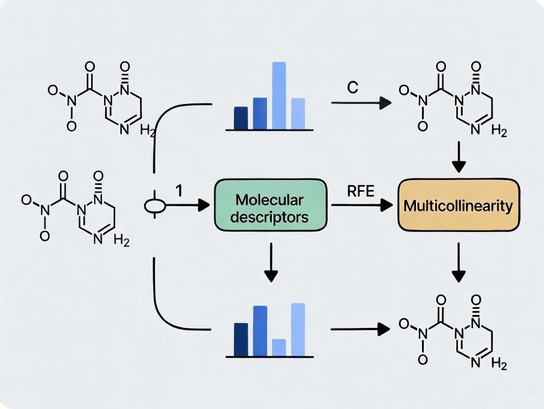
Robust QSAR Modeling: A Guide to Handling Multicollinearity in Molecular Descriptors for Recursive Feature Elimination

Abstract

Multicollinearity among molecular descriptors presents significant challenges for feature selection in QSAR modeling, particularly when using Recursive Feature Elimination (RFE). This comprehensive guide addresses the detection, mitigation, and validation strategies for handling descriptor intercorrelation to build more interpretable and generalizable predictive models. Covering foundational concepts through advanced applications, we explore Variance Inflation Factor (VIF) analysis, gradient boosting integration, and comparative performance evaluation across multiple molecular property prediction tasks. Targeted at researchers and drug development professionals, this article provides practical methodologies to enhance model robustness while maintaining predictive accuracy in cheminformatics and drug discovery applications.

Understanding Multicollinearity in Molecular Descriptors: Threats to QSAR Model Integrity

Defining Multicollinearity in the Context of Molecular Descriptors

Frequently Asked Questions

What is multicollinearity and why is it a problem in my research? Multicollinearity occurs when two or more independent variables in a model are highly correlated, meaning they share information and explain the same variance in the target variable [1]. In the context of molecular descriptors, this happens when descriptors like molecular weight, hydrophobicity, or the number of hydrogen bond donors/acceptors are not independent [2]. This correlation leads to:

• Unreliable and unstable estimates of regression coefficients, making it difficult to determine any one descriptor's individual impact on the model output [3] [1].
• Inflated standard errors for the coefficients of correlated features [1].
• Reduced model interpretability and poor generalization to new, unseen data [3] [1].

How does multicollinearity specifically affect Recursive Feature Elimination (RFE)? RFE is a feature selection method that iteratively removes the least important features to find an optimal subset [4]. Multicollinearity can destabilize this process because:

• The "importance" of a correlated feature can be misleading. If two descriptors are highly correlated, RFE might arbitrarily remove one, even though both carry similar information, leading to an unstable feature subset [4].
• The model's performance metric used to guide RFE can become unreliable due to the inflated variances caused by multicollinearity.

What are the most common methods to detect multicollinearity? You can use several diagnostic tools, often in combination [1]:

Method	Description	Interpretation / Threshold
Correlation Matrix	A table showing pairwise correlation coefficients between all features [3] [1].	Coefficients near +1 or -1 indicate high correlation [1].
Variance Inflation Factor (VIF)	Measures how much the variance of a feature's coefficient is inflated due to multicollinearity with other features [3] [1].	A VIF above 5 or 10 is a common rule-of-thumb for severe multicollinearity [4] [3] [1].
Condition Index	A scalar value reflecting the sensitivity of the model to small data changes [1].	A value above 30 suggests significant multicollinearity [1].
Tolerance	The inverse of VIF (Tolerance = 1/VIF) [3].	Values near 0 indicate a multicollinearity problem [1].

What are the best practices for handling multicollinearity in my dataset? There are multiple strategies, each with trade-offs between interpretability, simplicity, and model performance.

Strategy	Description	Best Used When
Remove Features [1]	Manually or automatically (e.g., via RFE) drop one or more correlated features.	You need a simple, interpretable model and can clearly identify redundant descriptors.
Transform Features [1]	Use Principal Component Analysis (PCA) to create new, uncorrelated features (components) that are linear combinations of the original ones.	Maintaining all information is critical, and you are willing to sacrifice some interpretability.
Regularize Features [1]	Apply Ridge Regression (shrinks coefficients but never to zero) or Lasso Regression (can shrink coefficients to zero, performing feature selection).	You want to retain all features while reducing the impact of multicollinearity and preventing overfitting.

Experimental Protocol: Diagnosing and Mitigating Multicollinearity

This protocol provides a step-by-step guide for a robust analysis of molecular descriptor data.

1. Data Pre-processing

• Calculate Molecular Descriptors: Use a cheminformatics platform (e.g., RDKit, alvaDesc, Dragon) to generate a wide array of numerical descriptors for your compound dataset [5].
• Scale Features: Standardize or normalize all descriptor values before analysis, as many methods (like regularization) are sensitive to variable scale [1].

2. Detection and Diagnosis

• Compute Correlation Matrix: Calculate the Pearson correlation matrix for all descriptors. Visualize it with a heatmap to quickly identify strongly correlated pairs (e.g., |r| > 0.8 or 0.9).
• Calculate VIF: For each descriptor, calculate the Variance Inflation Factor. A common practice is to iteratively remove the feature with the highest VIF above a threshold (e.g., 10) and recalculate until all VIFs are below the threshold [1].

3. Implementation of Mitigation Strategies

• Option A: Feature Removal via RFE
  • Use a supervised learning algorithm (e.g., Support Vector Machine with a linear kernel) as the estimator [4].
  • Specify the desired number of features (n_features_to_select) or let RFE determine it via cross-validation (RFECV).
  • Fit the RFE model to your data. The ranking_ attribute will show the order of feature elimination, and support_ will indicate the final selected features [4].
• Option B: Feature Transformation via PCA
  • Apply PCA to the scaled descriptor matrix.
  • Retain the top k principal components that explain a sufficient amount of the total variance (e.g., 95%).
  • Use these new, orthogonal components as features in your downstream predictive model.
• Option C: Feature Regularization via Ridge Regression
  • Standardize your features prior to modeling.
  • Use cross-validation to find the optimal value for the regularization strength hyperparameter (alpha or lambda).
  • Fit the Ridge regression model. The resulting coefficients will be more stable and reliable than those from a standard linear model.

The following workflow summarizes the key steps for diagnosing and treating multicollinearity:

The Scientist's Toolkit: Essential Research Reagents & Solutions

The following table lists key computational tools and their functions for handling multicollinearity in molecular descriptor research.

Tool / Solution	Function
Variance Inflation Factor (VIF)	A key diagnostic metric to quantify the severity of multicollinearity for each feature [3] [1].
Recursive Feature Elimination (RFE)	A wrapper method for feature selection that iteratively builds models and removes the weakest features to find an optimal subset [4].
Principal Component Analysis (PCA)	A dimensionality reduction technique that transforms correlated features into a set of linearly uncorrelated principal components [1].
Ridge Regression	A regularization technique that adds a penalty (L2 norm) to shrink coefficient estimates, improving stability under multicollinearity [3] [1].
Lasso Regression	A regularization technique (L1 norm) that can shrink some coefficients to zero, performing both feature selection and regularization [1].
Scikit-learn (Python)	A comprehensive machine learning library containing implementations for VIF, RFE, PCA, Ridge, and Lasso regression [4].
3-Methoxymollugin	3-Methoxymollugin, MF:C18H18O5, MW:314.3 g/mol
1(10)-Aristolen-2-one	1(10)-Aristolen-2-one, MF:C15H22O, MW:218.33 g/mol

FAQs on Descriptor Intercorrelation

What is descriptor intercorrelation and why is it a problem in QSAR modeling? Descriptor intercorrelation, also known as multicollinearity, occurs when two or more molecular descriptors in a dataset are highly correlated, meaning they provide redundant chemical information. This redundancy poses significant problems for QSAR modeling because it can inflate the variance of model parameter estimates, reduce model stability, and complicate the interpretation of which molecular features truly drive the observed activity or property. While some machine learning methods like Gradient Boosting are inherently more robust to collinearity, it remains a critical issue for many linear models and interpretability-focused studies [6] [7].

What are the common sources of this intercorrelation? Intercorrelation often arises from the fundamental nature of molecular structures. Common sources include:

• Constitutional Redundancy: Descriptors like molecular weight and the number of heavy atoms often scale together with the size of the molecule [8].
• Topological Connectivity: Different topological indices (e.g., Wiener Index, Balaban Index) calculated from the same molecular graph can capture overlapping aspects of molecular branching and connectivity [8] [9].
• Electronic Property Correlation: Electronic descriptors such as partial charges and the HOMO-LUMO gap can be influenced by common underlying electronic effects, leading to correlation [8].
• Descriptor Design: Many 1D, 2D, and 3D descriptors are derived from similar or related mathematical transformations of the molecular structure, inherently creating groups of correlated features [9].

How can I quickly check my dataset for descriptor intercorrelation? A correlation matrix is the most straightforward diagnostic tool. This matrix calculates the Pearson correlation coefficient for every pair of descriptors in your dataset. You can visualize it as a heatmap (Figure 1), where colors indicate the degree of correlation, allowing you to quickly identify highly correlated pairs or blocks of descriptors that may need to be addressed [6].

What is a reasonable correlation threshold for removing descriptors? There is no universally agreed-upon single threshold, as it can be dataset- and goal-dependent. However, studies have investigated the impact of different limits. The table below summarizes findings on how the number of retained descriptors changes with the correlation threshold and the subsequent effect on model performance [7].

Table 1: Impact of Intercorrelation Limits on Descriptor Count and Model Performance

Absolute Intercorrelation Limit	Effect on Number of Descriptors	Implication for Model Performance
0.80 - 0.90	Drastic reduction	May remove too many relevant descriptors, hurting performance.
0.95 - 0.97	Substantial reduction	Often a good balance for reducing redundancy.
0.99 - 0.995	Moderate reduction	Retains more descriptors; models may still suffer from multicollinearity.
1.000 (No limit)	No descriptors removed	High risk of overfitting and unreliable models.

Are certain types of machine learning models more resistant to intercorrelation? Yes. Tree-based ensemble methods like Gradient Boosting (e.g., XGBoost) and Random Forest are inherently more robust to descriptor intercorrelation. Their architecture, based on sequential splitting (boosting) or independent splitting (bagging) of features, naturally down-weights redundant descriptors, reducing the risk of overfitting to correlated noise [6] [10]. In contrast, models like Multiple Linear Regression (MLR) are highly sensitive to multicollinearity.

Troubleshooting Guide

Problem: Model is Overfitting

Symptoms

• Excellent performance on the training data but poor performance on the validation or test set.
• High variance in model coefficients when the training data is slightly perturbed.

Diagnosis and Solutions

• Generate a Correlation Matrix: Visually inspect the heatmap for large red or blue regions indicating groups of highly correlated descriptors [6].

• Apply a Variance Inflation Factor (VIF) Analysis: While not explicitly mentioned in the search results, VIF is a standard statistical measure for quantifying multicollinearity in linear models. It can be used alongside correlation analysis.
• Use Robust Algorithms: Switch to algorithms like Gradient Boosting Machines (GBM), which are less sensitive to intercorrelation. A case study on hERG inhibition showed that a GBM model significantly outperformed a linear model, in part due to its ability to handle complex, correlated descriptor relationships [6].
• Implement Advanced Feature Selection: Instead of simply filtering by correlation, use Recursive Feature Elimination (RFE). RFE is a wrapper method that iteratively builds a model and removes the least important features, considering the context of all other descriptors. This is a more sophisticated approach to handling redundancy [6] [10].

Problem: Model is Difficult to Interpret

Symptoms

• In a linear model, coefficients for correlated descriptors have counterintuitive signs or magnitudes.
• The "most important" features identified by the model change drastically with small changes in the training data.

Diagnosis and Solutions

• Systematic Feature Selection: Employ a method that systematically reduces feature multicollinearity. One proven approach involves:
  • Generating a large pool of molecular descriptors.
  • Iteratively identifying and removing one descriptor from each pair with a correlation above a chosen threshold (e.g., 0.95).
  • Using a genetic algorithm for variable selection to build a final, interpretable MLR model. This method has been shown to yield models with excellent performance while maintaining interpretability [11].
• Remove Constant and Low-Variance Descriptors: As a first step, filter out descriptors with constant values or very low variance across the dataset, as these contribute no meaningful information and can skew analysis [6] [12].

Experimental Protocol for Managing Intercorrelation

Objective: To preprocess a dataset of molecular descriptors to minimize the negative effects of intercorrelation prior to building a QSAR model, with a specific focus on preparing data for Recursive Feature Elimination (RFE).

Workflow: The following diagram outlines the logical sequence for diagnosing and managing descriptor intercorrelation.

Materials and Reagents: Table 2: Essential Computational Tools for Descriptor Management

Tool / Software	Type	Primary Function in this Protocol
RDKit	Open-Source Cheminformatics Library	Generation of 2D molecular descriptors and fingerprints [8].
DRAGON	Commercial Software	Generation of a wide range of molecular descriptors (2D, 3D) [7].
Python/R	Programming Languages	Calculation of correlation matrices, implementation of filtering scripts, and execution of RFE [6].
QSARINS	Software	Model building with Genetic Algorithm-based variable selection [7].
Flare Python API	Tool/API	Provides scripts for descriptor removal based on variance and multi-collinearity thresholds [6].

Methodology:

• Descriptor Generation and Initial Filtering:
  • Generate a comprehensive set of molecular descriptors using software like RDKit or DRAGON.
  • Remove all descriptors that are constant or have missing values across the dataset [7].
  • (Optional but recommended) Remove descriptors with very low variance, as they contain little useful information for modeling.

• Diagnosing Intercorrelation:

  • Compute a correlation matrix for all remaining descriptors.
  • Visually inspect the matrix using a heatmap to identify blocks of highly correlated descriptors.

• Applying a Correlation Filter:

  • Select an appropriate intercorrelation limit based on your modeling goals (see Table 1). For a balance between redundancy reduction and feature retention, a threshold between 0.95 and 0.97 is often effective [7].
  • Implement an algorithm to iterate through all descriptor pairs. For any pair with a correlation coefficient whose absolute value exceeds the threshold, remove the descriptor that has a higher average correlation with all other descriptors in the pool [7]. This process ensures a systematic reduction of the most redundant features.

• Advanced Feature Selection with RFE:

  • Use the filtered descriptor set from the previous step as input for Recursive Feature Elimination (RFE).
  • RFE will now work on a less redundant set, improving its efficiency and stability in identifying the most predictive, non-redundant features for the final model [6] [10].

Visual Guide to the Recursive Feature Elimination (RFE) Process

RFE is a powerful wrapper method for feature selection that works by recursively building a model and removing the weakest features until the desired number is reached. The following diagram illustrates this iterative process.

Frequently Asked Questions (FAQs)

Q1: What specific problems does multicollinearity create for RFE? Multicollinearity causes several critical issues for RFE-based feature selection:

• Unstable Feature Rankings: Correlated features can cause significant swings in feature importance scores, meaning the same feature might be ranked very differently with minor changes to the dataset or model parameters [13] [14].
• Misleading Elimination: RFE may incorrectly eliminate truly important causal variables because their importance is "shared" with correlated features, reducing their perceived contribution [14].
• Reduced Detection Power: In high-dimensional data, multicollinearity can decrease RFE's ability to detect true causal features, even when using specialized algorithms like Random Forest RFE (RF-RFE) [14].

Q2: How can I detect multicollinearity in my dataset before applying RFE? The primary method for detecting multicollinearity is calculating Variance Inflation Factors (VIF) [13] [15]:

• VIF Interpretation: A VIF value of 1 indicates no correlation, values between 1-5 show moderate correlation, and values greater than 5 indicate critical multicollinearity where coefficient estimates become unreliable [13].
• Correlation Matrices: Examine correlation matrices to identify pairs of features with high correlation coefficients, which can help visualize relationships between variables [16].

Q3: Does multicollinearity always require corrective action in RFE? Not necessarily—the need for action depends on your analysis goals [13]:

• Prediction-Focused Models: If the primary goal is prediction accuracy rather than interpretation, multicollinearity has minimal impact on the model's predictive capabilities [13].
• Interpretation-Focused Models: If understanding individual feature contributions is crucial, multicollinearity must be addressed to ensure reliable feature rankings and selections [13].

Q4: Can RFE handle datasets with many correlated molecular descriptors? Standard RFE struggles with highly correlated molecular descriptors. Research shows that in high-dimensional omics data (e.g., 356,341 variables), RF-RFE decreased the importance of both causal and correlated variables, making true signals harder to detect [14]. For such scenarios, consider supplementing RFE with preprocessing methods specifically designed to minimize multicollinearity [11] [17] [18].

Troubleshooting Guides

Problem 1: Unstable Feature Selection Results

Symptoms:

• Feature importance rankings change dramatically with small changes in the dataset
• Different features are selected when using different random seeds
• Inconsistent feature subsets across cross-validation folds

Solutions:

• Calculate VIF Scores: Quantify multicollinearity for all features using VIF [13] [15].
• Apply Correlation Analysis: Use correlation matrices to identify groups of highly correlated features [16].
• Implement Preprocessing: Center your variables to reduce structural multicollinearity, particularly when using interaction terms [13].
• Alternative Algorithms: For extremely high-dimensional data, consider that RFE may not scale well and explore alternative feature selection methods [14].

Problem 2: Important Features Being Incorrectly Eliminated

Symptoms:

• Known important features are ranked low and eliminated early
• Model performance decreases despite RFE selection
• Final feature subset lacks features with known biological significance

Solutions:

• Combine Filter Methods: Use statistical filter methods (e.g., correlation with target) before RFE to protect potentially important features [4].
• Adjust RFE Parameters: Use a smaller step size (eliminate fewer features per iteration) to make the elimination process more granular [19].
• Validate Externally: Compare selected features with domain knowledge to identify when important features are being lost [11].

Problem 3: Poor Model Performance After RFE

Symptoms:

• Model accuracy decreases after feature selection
• Selected features do not generalize to test datasets
• High variance in cross-validation performance

Solutions:

• Use Cross-Validation: Implement RFE within a cross-validation framework to ensure robust feature selection [4] [19].
• Pipeline Implementation: Ensure RFE and model training are properly encapsulated in a pipeline to prevent data leakage [19].
• Combine with Regularization: Use regularized models (e.g., Lasso) as the estimator within RFE to handle residual multicollinearity [4].

Experimental Data & Protocols

Quantitative Impact of Multicollinearity on RFE

Table 1: Performance Comparison of RF Models With and Without RFE in Presence of Multicollinearity

Metric	RF Without RFE	RF With RFE (RF-RFE)
R²	-0.00203	0.19217
MSEOOB	0.07378	0.05948
Causal SNP Detection	1 of 5 identified	Varied performance across SNPs
Causal CpG Detection	Poor	Poor
Computational Time	~6 hours	~148 hours

Data adapted from RF-RFE study on high-dimensional omics data [14]

VIF Threshold Guidelines for RFE Applications

Table 2: VIF Interpretation Guidelines for RFE Experiments

VIF Range	Multicollinearity Level	Recommended Action for RFE
1.0	None	No action needed
1.0-5.0	Moderate	Monitor but may not require intervention
>5.0	Critical	Address before RFE implementation
>10.0	Severe	Must be resolved for reliable RFE results

Based on multicollinearity analysis recommendations [13] [15]

Molecular Descriptor Selection Protocol

Objective: Systematically select molecular descriptors while minimizing collinearity for predictive modeling [11] [18]

Workflow:

• Descriptor Calculation: Generate comprehensive molecular descriptors from chemical structures
• Multicollinearity Screening: Calculate VIF for all descriptors and remove those with VIF > 5
• Initial RFE Implementation: Apply RFE with tree-based models to rank remaining features
• Iterative Refinement: Combine RFE with correlation analysis to select non-redundant, predictive features
• Validation: Verify selected features maintain predictive accuracy on holdout datasets

Key Considerations:

• Balance between feature importance and multicollinearity
• Domain knowledge integration to preserve scientifically meaningful features
• Computational efficiency for high-dimensional descriptor spaces [11]

Workflow Visualization

The Scientist's Toolkit: Research Reagent Solutions

Table 3: Essential Computational Tools for RFE with Molecular Descriptors

Tool/Technique	Primary Function	Application Context
Variance Inflation Factor (VIF)	Quantifies multicollinearity severity	Pre-RFE screening to identify problematic features [13] [15]
Correlation Matrix Analysis	Visualizes pairwise feature relationships	Identifying groups of correlated molecular descriptors [16]
Variable Centering/Standardization	Reduces structural multicollinearity	Essential when including interaction terms in models [13]
Tree-Based Pipeline Optimization (TPOT)	Automated machine learning pipeline optimization	Developing interpretable models with selected features [11]
Recursive Feature Elimination with Cross-Validation (RFECV)	Automated feature number selection	Determining optimal feature subset size while managing overfitting [4] [19]
Gradient-Boosted Feature Selection (GBFS)	Advanced feature selection workflow	Handling high-dimensional molecular descriptor spaces [18]
N-oleoyl alanine
Scutebata E	Scutebata E, MF:C28H40O9, MW:520.6 g/mol	Chemical Reagent

Frequently Asked Questions (FAQs)

1. What is multicollinearity and why is it problematic in molecular descriptor research? Multicollinearity occurs when two or more explanatory variables in a regression model are highly linearly intercorrelated [20]. In the context of molecular descriptor research, this means your descriptors are not independent, which inflates the variance of regression coefficients, leading to unreliable probability values and wide confidence intervals [20]. This makes it difficult to determine the individual effect of each molecular descriptor on your target property or activity, compromising the interpretability and statistical stability of your Quantitative Structure-Activity Relationship (QSAR) model [6].

2. How do I know which specific descriptors are multicollinear? While VIF and condition index can indicate the presence of multicollinearity, you need Variance Decomposition Proportions (VDP) to identify the specific variables involved [20]. When two or more VDPs, which correspond to a common condition index higher than 10 to 30, are higher than 0.8 to 0.9, their associated explanatory variables are considered multicollinear [20].

3. My model has high predictive power but also high multicollinearity. Should I be concerned? If your primary goal is only prediction, a model with high multicollinearity might still be usable [21]. However, for research aimed at understanding the unique contribution of each molecular descriptor (e.g., in Recursive Feature Elimination or RFE), multicollinearity is a critical issue. It masks the individual effect of descriptors, making it difficult to reliably select or eliminate features based on their importance [20] [6]. For interpretable models, correcting multicollinearity is essential.

4. Are some modeling techniques inherently robust to multicollinearity? Yes, machine learning models like Gradient Boosting are more resilient. Their decision-tree-based architecture naturally prioritizes informative splits and down-weights redundant descriptors, making them well-suited for high-dimensional descriptor sets with inherent correlations [6]. However, understanding descriptor intercorrelation remains vital for model interpretation and feature selection.

Troubleshooting Guides

Issue 1: Unstable Regression Coefficients and Inflated Standard Errors

Problem: The coefficients of your molecular descriptors change dramatically with small changes in the dataset, and their standard errors or confidence intervals are unusually large.

Diagnosis and Solution: This is a classic symptom of multicollinearity. Follow this diagnostic workflow to confirm and address the issue.

Detailed Diagnostic Protocol:

• Generate a Correlation Matrix

  • Objective: Visually identify pairs of descriptors with strong linear relationships.
  • Protocol: Create a table of Pearson's correlation coefficients for all pairs of molecular descriptors. Typically, a correlation greater than 0.80 or less than -0.80 indicates strong multicollinearity that requires further investigation [21]. Software like Python (with Pandas/Seaborn), R, or Displayr can be used to create and visualize this matrix [22].

• Calculate Variance Inflation Factors (VIF)

  • Objective: Quantify how much the variance of a regression coefficient is inflated due to multicollinearity.
  • Protocol:
    • For each descriptor X_i, run a multiple regression where X_i is the response variable and all other descriptors are the predictors.
    • Obtain the R-squared value (Ri²) from this regression.
    • Calculate VIF for X_i using the formula: VIF = 1 / (1 - Ri²) [23] [24].
    • A VIF of 1 indicates no multicollinearity. A VIF above 5 to 10 is generally considered problematic [20] [24].

• Perform Eigenanalysis (Condition Index and Variance Decomposition Proportions)

  • Objective: Identify the specific groups of descriptors that are multicollinear.
  • Protocol:
    • Standardize your explanatory variables and compute the correlation matrix.
    • Calculate the eigenvalues (λ) of this matrix.
    • Compute the Condition Index for each eigenvalue: √(λmax / λi). The largest condition index is the Condition Number [20].
    • Use the eigenvectors to calculate Variance Decomposition Proportions (VDPs), which show the proportion of variance each eigenvector contributes to each regression coefficient's variance [20].
    • Multicollinearity is indicated when two or more VDPs for different descriptors exceed 0.8-0.9 for a condition index greater than 10-30 [20].

Issue 2: High VIFs in a Model with Polynomial or Interaction Terms

Problem: You have included terms like X² or X*Y in your model to capture non-linearity, and these terms show extremely high VIFs.

Diagnosis and Solution: This is expected because X and X² are often highly correlated. This is a situation where high VIFs can sometimes be safely ignored because the model is correctly specified to capture a non-linear effect [24]. The solution is to center your variables (subtract the mean from each value of X) before creating the polynomial or interaction terms. This reduces the correlation between the linear and quadratic terms and can significantly lower the VIF, without changing the model's fundamental interpretation.

Diagnostic Metrics Reference Tables

Table 1: Interpretation Guidelines for Key Multicollinearity Diagnostics

Diagnostic Tool	Calculation	Acceptable Range	Problematic Range	Interpretation
Variance Inflation Factor (VIF)	( \text{VIF} = \frac{1}{(1 - R_i^2)} ) [23] [24]	1 - 5 [24]	5 - 10 or above [20] [21]	Factor by which the variance of a coefficient is inflated due to multicollinearity.
Tolerance	( \text{Tolerance} = 1 - R_i^2 ) [20]	0.2 - 1.0	0.1 - 0.25 or below [24]	Reciprocal of VIF. The amount of variance in a descriptor not explained by the others.
Condition Index (CI)	( \text{CI} = \sqrt{\frac{\lambda{max}}{\lambdai}} ) [20]	Below 10 - 15	10 - 30 or above [20]	Indates the presence of multicollinearity.
Variance Decomposition Proportion (VDP)	Derived from eigenvectors of the correlation matrix [20]	Below 0.8 - 0.9	Above 0.8 - 0.9 [20]	Identifies specific multicollinear variables when 2+ VDPs share a high CI.

Table 2: Summary of Correction Methods for Multicollinear Molecular Descriptors

Method	Procedure	Advantages	Disadvantages
Remove Variables	Manually remove one or more descriptors from a multicollinear group identified by VDP [20] [21].	Simple, improves model stability [20].	Risk of losing valuable information; requires domain knowledge [20].
Feature Selection (RFE)	Use Recursive Feature Elimination to iteratively remove the least important features based on model performance [6].	Data-driven; retains the most predictive features.	Computationally intensive; complex to implement.
Combine Variables	Create a composite index or score by averaging or summing highly correlated descriptors [21].	Reduces redundancy, preserves information.	May reduce interpretability of individual descriptors.
Regularization (Ridge Regression)	Use a biased estimation method that introduces a penalty term on large coefficients [20] [21].	Keeps all variables in the model; good for prediction.	Coefficients are biased, making interpretation less straightforward.
Switch to Robust ML Models	Use algorithms like Gradient Boosting that are inherently resilient to multicollinearity [6].	Handles multicollinearity automatically; powerful for prediction.	Model can be a "black box"; individual coefficient interpretation is difficult.

The Scientist's Toolkit: Essential Research Reagents & Solutions

Table 3: Key Resources for Multicollinearity Analysis in Molecular Research

Tool / Solution	Function / Description	Relevance to Multicollinearity
Statistical Software (R, Python)	Programming environments with extensive statistical and machine learning libraries (e.g., statsmodels, scikit-learn in Python).	Essential for calculating VIF, condition indices, performing PCA, and building regularized or Gradient Boosting models [6].
Molecular Descriptor Calculators (RDKit)	Open-source cheminformatics software that calculates a wide array of 2D and 3D molecular descriptors from chemical structures [6].	Generates the initial set of features that must be checked for intercorrelation before model building.
Flare V10 (Cresset)	An integrated platform for molecular modeling that includes QSAR capabilities and a Python API [6].	Provides scripts for descriptor removal based on variance and multicollinearity, and built-in robust Gradient Boosting models [6].
Gradient Boosting Machine Learning	A powerful tree-based ensemble algorithm that builds models sequentially to correct errors from previous trees [6].	A key solution, as it is inherently robust to multicollinearity, reducing the need for extensive pre-filtering of descriptors [6].
Principal Component Analysis (PCA)	A dimensionality-reduction technique that transforms original variables into a new set of uncorrelated components [21] [24].	A corrective measure used to create a smaller set of uncorrelated variables from a large number of multicollinear descriptors.
Agistatin D	(4aR,5R,6R)-6-Ethyl-4a,5-dihydroxy-4a,5,6,7-tetrahydro-4H-1-benzopyran-4-one|Agistatin D	High-purity (4aR,5R,6R)-6-Ethyl-4a,5-dihydroxy-4a,5,6,7-tetrahydro-4H-1-benzopyran-4-one (Agistatin D) for research. This product is For Research Use Only. Not for human or veterinary diagnostic or therapeutic use.
Homalomenol A	Homalomenol A|CAS 145400-03-9|Sesquiterpenoid	Homalomenol A is a natural sesquiterpenoid for inflammation research. For Research Use Only. Not for human or veterinary diagnostic or therapeutic use.

In the context of building robust Quantitative Structure-Activity Relationship (QSAR) models for drug discovery, managing multicollinearity within molecular descriptor sets is a critical pre-processing step. Multicollinearity occurs when two or more predictor variables in a dataset are highly correlated, which can lead to unstable model coefficients, inflated standard errors, and reduced statistical power, ultimately compromising the interpretability and reliability of your models [15] [6] [25]. This case study, framed within broader thesis research on handling multicollinearity for Recursive Feature Elimination (RFE), provides a technical guide for researchers and scientists encountering these issues during their experiments with RDKit descriptors.

---

Troubleshooting Guides & FAQs

FAQ 1: Why does multicollinearity pose a problem for my QSAR model and subsequent RFE?

Multicollinearity is problematic because it undermines the statistical integrity of your regression-based QSAR models and can confound the feature selection process.

• Unstable Coefficient Estimates: When predictors are highly correlated, the regression coefficients can become highly sensitive to minor changes in the model or the data, making their values unreliable [25].
• Reduced Statistical Power: It becomes harder to detect significant relationships between individual descriptors and the target response variable [25].
• Inflated Standard Errors: This leads to wider confidence intervals and less precise estimates of the coefficients [15] [25].
• Impact on RFE: While wrapper methods like RFE consider feature interactions [4], a dataset plagued by multicollinearity can cause the algorithm to be unstable in its initial rankings, potentially leading to the arbitrary elimination of important features.

FAQ 2: How can I detect multicollinearity in my set of RDKit descriptors?

A multi-faceted approach is recommended to reliably diagnose multicollinearity. The following workflow outlines a robust diagnostic protocol:

Experimental Protocol for Diagnosis:

• Calculate the Feature Correlation Matrix

  • Methodology: Using Python's pandas library, compute the Pearson correlation coefficient for every pair of descriptors in your dataset. This generates a matrix where each cell shows the correlation between two variables.
  • Interpretation: Visually inspect the matrix using a heatmap. Look for pairs of descriptors with correlation coefficients exceeding a predetermined threshold, typically |r| > 0.8 or |r| > 0.9 [6] [25].

• Compute the Variance Inflation Factor (VIF)

  • Methodology: For each descriptor X_i, run an ordinary least squares regression where X_i is the dependent variable predicted by all other descriptors in the set. The VIF is then calculated as VIF = 1 / (1 - R²_i), where R²_i is the coefficient of determination from that regression.
  • Interpretation: Use the following table to assess the severity of multicollinearity based on the VIF values [15] [25]:

VIF Value	Interpretation
VIF = 1	No multicollinearity
1 < VIF ≤ 5	Moderate multicollinearity
5 < VIF ≤ 10	High multicollinearity; potential issue
VIF > 10	Severe multicollinearity; requires remediation [25]

FAQ 3: What are the best practices for handling multicollinearity before applying RFE?

Once multicollinearity is diagnosed, you can apply several strategies to mitigate its effects. The table below compares the most common approaches.

Method	Brief Explanation	Key Consideration for QSAR
Remove Correlated Features	Manually remove one descriptor from each highly correlated pair (based on correlation matrix or VIF) [6] [25].	Simple and effective, but may discard chemically relevant information if done without domain knowledge.
Use Regularization	Apply Ridge Regression (L2 penalty) or Lasso (L1 penalty), which constrains coefficient sizes and handles correlated variables well [15] [25].	Improves model stability and prediction; Lasso can also perform feature selection by zeroing some coefficients.
Principal Component Analysis (PCA)	Transform original correlated descriptors into a smaller set of linearly uncorrelated principal components [4] [25].	Preserves variance while eliminating multicollinearity, but the new features lose chemical interpretability.
Leverage Robust Algorithms	Use tree-based models like Gradient Boosting or Random Forest, which are inherently less sensitive to multicollinearity [6].	Algorithms like XGBoost can naturally prioritize important features and are less prone to overfitting [6].

FAQ 4: My RFE model is overfitting even after removing correlated features. What else can I do?

Overfitting occurs when a model learns the noise in the training data rather than the underlying pattern. If basic multicollinearity handling isn't sufficient, consider these advanced protocols:

• Refine Your RFE Protocol:

  • Use RFECV: Implement Recursive Feature Elimination with Cross-Validation (RFECV) to automatically determine the optimal number of features, which helps in preventing overfitting by evaluating feature subsets on different validation folds [4].
  • Pipeline Integration: Always embed the RFE and your final model within a scikit-learn Pipeline and perform hyperparameter tuning and validation on this entire pipeline. This prevents data leakage and ensures a more realistic performance estimate [19].

• Apply Stronger Regularization: If using linear models, increase the regularization strength (e.g., the alpha parameter in Ridge or Lasso regression). This more heavily penalizes large coefficients, simplifying the model [25].

• Tune Model Hyperparameters: For tree-based models, limit model complexity by tuning hyperparameters such as maximum tree depth, minimum samples per leaf, and learning rate (for boosting algorithms) to reduce variance [6].

---

The Scientist's Toolkit: Essential Research Reagents & Solutions

The following table details key software and libraries essential for implementing the protocols described in this case study.

Item Name	Function / Application
RDKit	A core open-source cheminformatics toolkit used to calculate 1D, 2D, and 3D molecular descriptors from chemical structures [9].
Scikit-learn	A fundamental Python library for machine learning. It provides the RFE and RFECV classes, various models, and preprocessing tools [4] [19].
Statsmodels & SciPy	Libraries offering comprehensive statistical functions, including the calculation of Variance Inflation Factors (VIF) and correlation matrices.
DOPtools	A specialized Python platform that provides a unified API for calculating chemical descriptors and is especially suited for reaction modeling [26].
Pandas & NumPy	Core Python libraries for data manipulation, analysis, and numerical computations, essential for handling descriptor matrices.
6-Ethoxy-5-methylnicotinaldehyde	6-Ethoxy-5-methylnicotinaldehyde|CAS 1224604-16-3
Dihydroobovatin	Dihydroobovatin

Integrated RFE Workflows: Combining Statistical and Machine Learning Approaches

For researchers in drug development working with molecular descriptors, pre-processing data is a critical step to ensure robust model performance. Techniques like centering, scaling, and initial filtering are foundational for mitigating multicollinearity—a common issue where correlated predictors inflate model variance and obscure the true effect of individual molecular features. This guide provides targeted troubleshooting advice to address specific challenges encountered when preparing data for advanced feature selection methods like Recursive Feature Elimination (RFE).

---

Frequently Asked Questions (FAQs)

FAQ 1: Why should I center and scale my molecular descriptor data before using RFE? Many machine learning algorithms, including those used in RFE, are sensitive to the scale of your features. Molecular descriptors often contain integer, decimal, and binary values on vastly different scales [17]. If one descriptor has a much larger scale (e.g., molecular weight in the hundreds) than another (e.g., a binary indicator), the model may incorrectly perceive it as more important [27]. Centering and scaling ensure all features contribute equally, which is crucial for distance-based models like Support Vector Machines (SVMs)—a common choice for RFE—and gradient-based models to converge effectively [4] [27].

FAQ 2: My model's coefficients are highly unstable and change drastically when I add or remove a variable. What is happening? This is a classic symptom of multicollinearity, where independent variables in your regression model are highly correlated [13] [25]. When descriptors are correlated, it becomes difficult for the model to isolate each one's individual effect on the response variable. This leads to unreliable coefficient estimates, inflated standard errors, and reduced statistical power, making it hard to identify truly significant molecular features [13] [25].

FAQ 3: How can I detect multicollinearity in my dataset of molecular descriptors? The most straightforward method is to calculate the Variance Inflation Factor (VIF) for each descriptor.

• VIF = 1: No multicollinearity.
• 1 < VIF ≤ 5: Moderate correlation, often acceptable.
• VIF > 5 to 10: High multicollinearity that needs attention [13] [25]. You can also examine a correlation matrix to identify pairs of descriptors with high correlation coefficients [25].

FAQ 4: I have high multicollinearity, but I need to keep all my descriptors for interpretation. What can I do? If your primary goal is prediction rather than interpretation, you can use regularization techniques like Ridge Regression [25]. Ridge regression adds an L2 penalty to the model's coefficients, which shrinks them but does not set any to zero. This helps stabilize the coefficient estimates and mitigate the effects of multicollinearity without removing any features [25].

FAQ 5: Does multicollinearity affect my model's predictive accuracy? Not necessarily. Multicollinearity primarily affects the interpretation of individual coefficients and their p-values. Your model's overall predictions, R-squared value, and goodness-of-fit statistics may remain unaffected [13]. Therefore, if your only goal is to make accurate predictions, severe multicollinearity may not always be a critical problem.

---

Troubleshooting Guides

Issue: High Multicollinearity Detected by VIF

Problem: The VIF for several molecular descriptors is above the acceptable threshold (e.g., VIF > 5), indicating severe multicollinearity [13] [25].

Solution: Apply one or more of the following strategies.

Table 1: Strategies for Remediating High Multicollinearity

Strategy	Description	Best For	Considerations
Remove Correlated Features	Identify and remove one of the highly correlated descriptors.	Simplicity; when interpretability is key.	You may lose information from the removed feature.
Principal Component Analysis (PCA)	Transform correlated variables into a new set of uncorrelated principal components.	High-dimensional datasets; when prediction is the main goal.	New components are less interpretable than original descriptors.
Ridge Regression	Apply a regularization penalty (L2) that shrinks coefficients but keeps all features.	When you need to keep all descriptors for interpretation.	Coefficients are biased but more stable.

Experimental Protocol: Using PCA to Handle Multicollinearity This protocol uses scikit-learn to reduce descriptor correlation.

• Standardize the Data: PCA is affected by feature scale, so you must center and scale the data first [28].

• Apply PCA: Transform the standardized data into principal components.

• Check Explained Variance: Determine how much information the new components retain.
  The resulting X_pca can be used as input for your RFE model [25].

Issue: Model Performance is Poor or Inconsistent After Pre-processing

Problem: After centering, scaling, and feature filtering, the model's performance does not improve or becomes worse.

Solution: Review your pre-processing sequence and model selection.

• Data Leakage: Ensure that scaling and feature selection are fit only on the training data. Use a Pipeline to prevent information from the test set leaking into the training process [28].

• Incorrect Scaler for Data Type: Use MaxAbsScaler for data that is already centered at zero or sparse data, as centering sparse data would destroy its structure [28].
• Algorithm Choice: Remember that not all models require scaling. Tree-based models (e.g., Random Forests) are insensitive to feature scale, so pre-processing may be an unnecessary step for them [27].

Table 2: Comparison of Common Scaling Methods

Method	Formula	Use Case	Advantages	Disadvantages
Standardization (Z-score)	(X - μ) / σ	PCA, SVMs, linear models.	Results in a standard normal distribution.	Sensitive to outliers.
Min-Max Scaling	(X - Xmin) / (Xmax - X_min)	Neural networks, data bounded in a range.	Preserves original data distribution.	Also sensitive to outliers.
MaxAbs Scaling	X /	X_max		Sparse data.	Preserves sparsity and sign of data.	Not suitable if data is not centered.

---

Workflow and Process Diagrams

Diagram 1: Pre-processing and Feature Selection Workflow This diagram outlines the logical sequence for handling molecular descriptor data, from raw data to a refined feature set ready for modeling.

Diagram 2: The Recursive Feature Elimination (RFE) Process This diagram details the iterative loop at the heart of the RFE algorithm for feature selection.

---

The Scientist's Toolkit

Table 3: Essential Software and Libraries for Pre-processing

Tool / Library	Function	Application in Pre-processing
scikit-learn [28] [29]	A comprehensive machine learning library for Python.	Provides StandardScaler, MinMaxScaler, VarianceThreshold, RFE, PCA, and Ridge regression, making it a one-stop shop for all pre-processing and modeling steps.
RDKit [30]	An open-source cheminformatics toolkit.	Used to generate canonical molecular descriptors and fingerprints from SMILES strings, which form the initial raw feature set.
Mordred [30]	A molecular descriptor calculator.	Can generate a very extensive set of over 1,600 molecular descriptors for a comprehensive feature space.
Python (NumPy, pandas)	Programming language and data manipulation libraries.	The foundation for data handling, manipulation, and orchestrating the entire pre-processing workflow.
Dehydroformouregine	Dehydroformouregine|High-Purity Research Compound	Dehydroformouregine is an N-formyl aporphine alkaloid for research use only (RUO). It is strictly for laboratory applications and not for human or veterinary use.
Honyucitrin	Honyucitrin, CAS:114542-44-8, MF:C25H26O5, MW:406.5 g/mol	Chemical Reagent

Frequently Asked Questions (FAQs)

Q1: What is the primary advantage of using GBFS over other feature selection methods for molecular data?

GBFS is a novel feature selection algorithm that satisfies four key conditions ideal for molecular data: it reliably extracts relevant features, can identify non-linear feature interactions, scales linearly with the number of features and dimensions, and allows for the incorporation of known sparsity structure. Its flexibility and scalability make it particularly well-suited for high-dimensional molecular descriptor datasets [31].

Q2: My model performance is good, but the selected molecular descriptors seem biased towards categorical variables with high cardinality. How can I address this?

This is a known issue with standard Gradient Boosting Machines (GBM); their base learners can be biased towards categorical variables with many categories, which can skew feature importance measures. To mitigate this, implement a Cross-Validated Boosting (CVB) framework. In CVB, a variable is selected for splitting based on its cross-validated performance rather than its performance on the training sample alone. This ensures a "fair" comparison between features and leads to more reliable feature importance scores while maintaining predictive accuracy [32].

Q3: How can I improve the stability of my selected feature set when using Recursive Feature Elimination (RFE) with molecular data?

Stability in feature selection can be significantly improved by applying a data transformation before RFE. Specifically, research in microbiome data (which shares high-dimensional characteristics with molecular descriptor data) has shown that using a kernel-based transformation, such as one derived from the Bray–Curtis similarity matrix, before RFE can substantially improve the stability of the selected features without sacrificing classification performance. This method projects data into a new space where correlated features are mapped closer together, making the selection process more robust [33].

Q4: Are there hybrid methods that combine GBFS with other feature selection techniques for better results?

Yes, hybrid methods are highly effective. You can combine the power of GBFS with the precision of Recursive Feature Elimination with Cross-Validation (RFECV). For instance, a pipeline can be designed where a Gradient Boosting Machine (GBM) is used as the core estimator within the RFECV process (RFECV-GBM). This hybrid approach leverages the GBM's ability to model complex relationships to recursively eliminate the least important features in a cross-validated manner, ensuring an optimal and robust subset of features is selected [34].

Q5: Is there a systematic way to select molecular descriptors to minimize multicollinearity?

A proven method involves systematically selecting molecular descriptor features to reduce feature multicollinearity. This process simplifies feature selection by minimizing redundant information between descriptors. The resulting models are not only interpretable but also maintain high performance, enabling the discovery of new, robust relationships between global molecular properties and their descriptors [11].

Troubleshooting Guides

Issue 1: Poor Model Generalization Despite High Training Accuracy

Symptoms:

• High performance on training data but significant drop in performance on validation or test sets.
• Selected feature set varies greatly with slight changes in the training data.

Possible Causes and Solutions:

• Cause 1: High Multicollinearity Among Molecular Descriptors.

  • Solution: Implement a pre-processing step to reduce feature multicollinearity. Systematically select descriptors to minimize collinearity before applying GBFS or RFE. This improves model interpretability and stability [11].
  • Actionable Step: Calculate the correlation matrix for your molecular descriptors. Use variance inflation factors (VIF) or a similar metric to identify and remove highly correlated descriptors prior to feature selection.

• Cause 2: Unstable Feature Selection.

  • Solution: Use a hybrid RFECV method with a robust base estimator like GBM or Random Forest. RFECV provides a more stable feature ranking through cross-validation [35] [34].
  • Actionable Step: Employ the RFECV function from ML libraries (e.g., scikit-learn) using a GradientBoostingClassifier or GradientBoostingRegressor as the estimator. This will output a cross-validated ranking of your features.

Issue 2: Biased Feature Importance from Categorical Descriptors

Symptoms:

• Categorical molecular descriptors (e.g., functional group presence, atom types) with a large number of categories are consistently ranked as the most important, even when domain knowledge suggests otherwise.

Possible Causes and Solutions:

• Cause: Inherent bias in standard GBM implementations towards high-cardinality categorical features.
  • Solution: Implement Cross-Validated Boosting (CVB) to correct the bias in feature importance measures [32].
  • Actionable Step: Instead of using a standard GBM, modify the tree-growing process. During training, for each split, evaluate a feature's performance using k-fold cross-validation on the training data at that node. Select the feature with the best generalizable performance.

Issue 3: Computationally Expensive Feature Selection

Symptoms:

• The feature selection process takes an impractically long time for large-scale molecular datasets with thousands of descriptors.

Possible Causes and Solutions:

• Cause: The wrapper method (like RFE) requires retraining the model multiple times, which is computationally heavy.
  • Solution 1: Leverage the inherent efficiency of the GBFS algorithm, which is designed to scale linearly with the number of features and dimensions [31].
  • Solution 2: Use stochastic modifications of GBM, such as those in LightGBM or XGBoost, which use sampling techniques to speed up the training process of each base learner [32].
  • Actionable Step: For large datasets, use implementations like LightGBM, which supports categorical features natively and uses histogram-based algorithms for faster training, as the core estimator in your GBFS or RFECV pipeline.

Experimental Protocols & Workflows

Detailed Methodology: Systematic Descriptor Selection and Modeling

The following protocol, adapted from a study on biofuel molecular properties, outlines a robust pipeline for building interpretable models with selected molecular descriptors [11].

• Data Collection: Assemble a publicly available experimental dataset for the target molecular property (e.g., melting point, boiling point). The study used up to 8,351 organic molecules.
• Descriptor Calculation: Compute a comprehensive set of molecular descriptors for all molecules in the dataset.
• Feature Selection & Multicollinearity Reduction: Apply a systematic method for selecting molecular descriptor features to minimize feature multicollinearity.
• Model Training with AutoML: Use the Tree-based Pipeline Optimization Tool (TPOT) to train and select the best-performing model architecture on the selected features.
• Performance Evaluation: Evaluate the final model using metrics like Mean Absolute Percent Error (MAPE). The cited study achieved MAPE values ranging from 3.3% to 10.5% for various properties.
• Interpretation and Tool Deployment: Analyze the set of features that are well-correlated with the property. Integrate the data and models into an open-source, interactive web tool for broader use.

GBFS Hybrid Workflow Diagram

The diagram below illustrates a hybrid feature selection workflow that combines GBFS and RFECV for robust feature selection on molecular data.

Research Reagents & Computational Tools

Table 1: Essential Materials and Tools for a GBFS Workflow

Item	Function/Description	Relevance to GBFS Workflow
TPOT (Tree-based Pipeline Optimization Tool)	An AutoML tool that automates the process of model selection and hyperparameter tuning using genetic programming.	Used to train and optimize the final predictive models after feature selection, ensuring high performance without manual tuning [11].
LightGBM (LGBM)	A gradient boosting framework that uses tree-based algorithms and supports categorical features directly. It is optimized for high speed and efficiency.	Can serve as a high-performance base learner for GBFS or within an RFECV pipeline, especially with large datasets and categorical molecular descriptors [32].
XGBoost	An optimized distributed gradient boosting library designed to be efficient and flexible.	A common choice for implementing the core boosting algorithm in GBFS, known for its regularization and scalability [32] [34].
RFECV (Recursive Feature Elimination with Cross-Validation)	A wrapper method that recursively removes the least important features based on a model's feature importance, using cross-validation to determine the optimal number of features.	Forms the basis of a hybrid approach (e.g., RFECV-GBM) to create a stable and optimal feature subset [35] [34].
Bray-Curtis Similarity / UMAP	A data transformation technique that projects features into a new space based on similarity, improving the stability of subsequent feature selection.	Applied before RFE to improve the stability and reliability of the selected molecular descriptors [33].

Implementing RFE with Stability Enhancements for Correlated Descriptors

Frequently Asked Questions

Q1: Why does my feature selection become unstable when I run Recursive Feature Elimination (RFE) on a dataset with highly correlated molecular descriptors?

Highly correlated descriptors create instability in RFE because the algorithm may arbitrarily select one correlated feature over another during its iterative elimination process, as both carry similar predictive information. This can lead to different feature subsets being selected across different runs or data splits, reducing the reproducibility of your model. Implementing a pre-filtering step to reduce multicollinearity before applying RFE is recommended to enhance stability [36] [6].

Q2: What are the practical methods to pre-filter correlated descriptors to stabilize RFE output?

A highly effective method is to first calculate the correlation matrix for all descriptors and then filter them based on a pre-defined threshold (e.g., |r| > 0.8). From each group of highly correlated features, you can retain only the one with the highest correlation to the target property, removing the others. This process reduces redundancy and the arbitrary influence of correlated feature groups on the RFE algorithm, leading to more stable and interpretable feature subsets [36] [6].

Q3: My model performance drops after removing correlated descriptors. Is this normal, and how can I mitigate it?

This can occur if the removed descriptors, while redundant, still contained subtle, unique information. However, this performance drop is often minimal and is counterbalanced by significant gains in model stability and generalizability. To mitigate the drop, consider using machine learning models like Gradient Boosting (GB) or Random Forest (RF), which are inherently more robust to multicollinearity. Their tree-based structure naturally down-weights redundant features, making them ideal for use with RFE on descriptor sets where some correlation may remain [6].

Q4: How can I validate that my stabilized RFE process is truly reproducible?

To validate reproducibility, you should run the entire stabilized pipeline—including correlation filtering and RFE—multiple times using different random seeds for data splitting (e.g., in k-fold cross-validation). A stable process will yield a highly consistent set of selected features across these iterations. You can quantify this stability using metrics like the Jaccard index, which measures the similarity between the feature subsets selected in different runs [36].

Detailed Experimental Protocol

The following workflow, termed the Stabilized RFE (S-RFE) Pipeline, integrates correlation filtering with RFE to ensure robust feature selection from a high-dimensional descriptor space.

Stabilized RFE (S-RFE) Workflow

Phase 1: Data Preprocessing and Correlation Filtering

• Descriptor Calculation and Initial Cleaning: Calculate a comprehensive set of molecular descriptors (e.g., using RDKit) for all compounds in your dataset. Remove descriptors with zero variance or a high proportion of missing values [6].
• Construct Correlation Matrix: Calculate the pairwise Pearson correlation coefficient for all remaining descriptors. Visualize the matrix to identify blocks of highly correlated features [6].
• Apply Correlation Filter:
  • Set a correlation threshold (commonly |r| > 0.8 or 0.9).
  • Identify clusters of descriptors that exceed this threshold.
  • Within each cluster, calculate the absolute correlation between each descriptor and the target property (e.g., biological activity, retention time).
  • Retain only the descriptor with the highest absolute correlation to the target and remove the others from the dataset [36].
  • This results in a reduced, less redundant descriptor set.

Phase 2: Stabilized Recursive Feature Elimination

• Algorithm Selection: Select a base estimator for RFE. Tree-based models like Gradient Boosting (GB) or Random Forest (RF) are preferred as they are robust to any residual multicollinearity. Alternatively, a linear model like SVM can be used for a more aggressive feature selection approach [6] [10].
• Iterative Feature Elimination:
  • The RFE process is run on the pre-filtered descriptor set.
  • The model is trained, and feature importance are assessed.
  • The least important features (e.g., bottom 10-20%) are pruned.
  • The process repeats with the remaining features until the predefined number of features is reached.
• Cross-Validation Integration: To ensure robustness, the entire S-RFE pipeline should be performed within a cross-validation loop (e.g., 5-fold or 10-fold). This prevents data leakage and provides a realistic assessment of the model's performance and the stability of the selected features on unseen data [36].

Phase 3: Validation and Final Model Training

• Stability Assessment: Compare the feature subsets selected across different cross-validation folds. A high degree of overlap indicates a stable feature selection process.
• Final Model Training: Using the stable feature subset identified by the S-RFE pipeline, train a final model on the entire training set. Validate its performance on a held-out test set that was not used at any stage of the feature selection process [10].

The table below summarizes the typical outcomes of applying the S-RFE pipeline compared to standard RFE, as evidenced by related research.

Table 1: Performance Comparison of Standard RFE vs. Stabilized RFE (S-RFE) Pipeline

Metric	Standard RFE	S-RFE Pipeline (with Correlation Filtering)	Context / Model
Feature Set Stability	Low to Moderate	High	Parkinson's disease detection with XGBoost [36]
Model Generalizability	Can be reduced due to overfitting	Improved	QSAR modeling with Gradient Boosting [6]
Final Model Accuracy	96.1% ± 0.8%	98.3% ± 0.8%	Subject-wise PD detection, XGBoost [36]
Number of Final Features	Often larger and redundant	Reduced and informative	Molecular property prediction [11]
Computational Cost	Lower per iteration, but may require more runs	Slightly higher initial cost, more efficient long-term	General QSRR modeling [10]

The Scientist's Toolkit

Table 2: Essential Research Reagents & Computational Tools

Item / Resource	Function in S-RFE Pipeline	Implementation Notes
RDKit	Calculates 2D and 3D molecular descriptors from chemical structures.	Used to generate physicochemical properties, topological indices, and fingerprints as the initial feature pool [6].
scikit-learn (Python)	Provides implementations for RFE, correlation analysis, and various ML models (GB, RF, SVM).	The RFE and SelectFromModel classes are key. Integration with Pipeline ensures a proper workflow [36] [10].
Gradient Boosting Models (XGBoost, GBR)	Acts as the base estimator for RFE; robust to residual multicollinearity.	Provides feature importance scores for the elimination process. XGBoost has been shown to deliver high performance in stabilized pipelines [36] [6].
Correlation Threshold	A user-defined value (e.g., 0.8-0.9) to identify and filter redundant descriptors.	A critical parameter; a higher value retains more features, while a lower value creates a more aggressive filter [36] [6].
k-fold Cross-Validation	Evaluates the stability and generalizability of the selected feature subset.	Prevents overfitting and provides a realistic performance estimate for the final model [36] [10].
Agistatin E	Agistatin E, MF:C11H16O5, MW:228.24 g/mol	Chemical Reagent

Integration with Gradient Boosting Models for Inherent Multicollinearity Resistance

Gradient Boosting Models (GBMs), including advanced implementations like XGBoost, are highly regarded in quantitative structure-activity relationship (QSAR) studies and molecular descriptor research for their inherent resistance to multicollinearity. Unlike linear models that can become unstable and produce unreliable coefficient estimates when predictors are highly correlated, tree-based boosting algorithms make splitting decisions based on one feature at a time. This process naturally avoids the pitfalls of multicollinearity, as the model prioritizes the most predictive features regardless of their correlation with others [37] [38]. Furthermore, GBMs possess built-in regularization mechanisms that prevent overfitting and enhance generalization to new data, making them particularly robust for high-dimensional biological data where correlated features are common [38] [39].

Frequently Asked Questions (FAQs)

Q1: Why should I choose Gradient Boosting over Linear Regression (like LASSO) for my dataset with highly correlated molecular descriptors?

Linear models, including penalized versions like LASSO regression, are highly sensitive to multicollinearity. This can lead to inflated coefficient variances and unstable feature selection, making model interpretation difficult [40] [39]. In contrast, Gradient Boosting is a tree-based ensemble method that makes decisions based on one feature at a time. This fundamental characteristic makes it inherently robust to correlated descriptors, as it can use whichever predictor provides the best split at a given node. While it may not automatically exclude redundant features, it effectively manages them without compromising predictive accuracy [37] [38].

Q2: A highly correlated descriptor was ranked as very important by my GBM. Should I manually remove the other correlated descriptors it's linked to?

Not necessarily. The GBM's feature importance score reflects a feature's utility in the model's prediction, even in the presence of correlation. If a descriptor is ranked as highly important, it means the model consistently finds it valuable for making splits. Manually removing its correlated counterparts could harm performance if those features provide complementary information in different contexts of the tree. It is often better to trust the model's selection unless you have a specific scientific reason (e.g., domain knowledge) to do otherwise [11].

Q3: My GBM model has high predictive accuracy on the training data but performs poorly on the test set. What could be the cause and how can I fix it?

This is a classic sign of overfitting. While GBMs are robust to multicollinearity, they can still overfit, especially with noisy data or improper hyperparameter settings [39]. To address this:

• Tune Hyperparameters: Key parameters to adjust are the learning rate (eta in XGBoost), the maximum depth of the trees (max_depth), and the number of boosting rounds (n_estimators). A lower learning rate with a higher number of trees often leads to better generalization [41].
• Increase Regularization: Modern GBMs like XGBoost offer L1 and L2 regularization terms on the weights of the model. Increasing these parameters can penalize complexity and reduce overfitting [39].
• Use Early Stopping: Implement early stopping during training to halt the process when the performance on a validation set stops improving, thus preventing the model from learning the noise in the training data [41].

Q4: How can I improve the interpretability of my GBM model to understand which molecular descriptors are most critical?

Although GBMs are often seen as "black boxes," several techniques can aid interpretation:

• Feature Importance: GBMs natively provide a feature importance score based on how much a feature improves the model's performance (e.g., "gain" in XGBoost). This is an excellent starting point for identifying the most influential descriptors [41] [11].
• SHAP (SHapley Additive exPlanations) Values: SHAP is a game-theoretic approach that assigns each feature an importance value for a single prediction. It provides a unified and more consistent measure of feature impact than traditional importance scores and can be visualized in various plots (e.g., summary plots, dependence plots) to deepen your understanding [41].

Experimental Protocols & Validation

Protocol 1: Validating GBM's Robustness to Multicollinearity

This protocol outlines a comparative experiment to benchmark GBM's performance against other algorithms in the presence of multicollinearity.

1. Objective: To compare the predictive performance and stability of Gradient Boosting, Linear Regression, and Random Forest when trained on a dataset of highly correlated molecular descriptors. 2. Dataset: * Utilize a publicly available dataset of known HIV integrase inhibitors, such as the one from the ChEMBL database [42]. * Calculate a standard set of molecular descriptors (e.g., Molecular Weight, LogP, Hydrogen Bond Donors/Acceptors, Topological Polar Surface Area) [42] [11]. 3. Introducing Multicollinearity: * Compute the correlation matrix for all molecular descriptors. * Artificially engineer new, highly correlated variables (e.g., LogP_x_1.1, TPSA + 0.1*MW) to augment the dataset and simulate a high-collinearity environment. 4. Model Training & Comparison: * Models: Train a GBM (e.g., XGBoost), a Linear Regression model with L2 regularization (Ridge), and a Random Forest. * Feature Selection: Apply Recursive Feature Elimination (RFE) with each model to identify the most predictive descriptors [42] [41]. * Evaluation: Use a hold-out test set or cross-validation. Record key performance metrics and the final set of selected features for each model.

Table 1: Expected Performance Metrics in a High-Multicollinearity Scenario

Model	Expected RMSE	Expected Accuracy/Precision	Feature Selection Stability
Gradient Boosting (XGBoost)	Low (e.g., ~0.82 AUC) [42]	High (e.g., ~0.79 Precision) [42]	High
Ridge Regression	Moderate	Moderate	Low (coefficients shrink but all features retained)
Random Forest	Low [41]	High [41]	Moderate (can be affected by correlated features)

Protocol 2: A Systematic Workflow for Molecular Descriptor Selection with GBM

This workflow integrates GBM with systematic feature selection for building robust QSAR models.

1. Data Curation: Source and clean bioactivity data (e.g., IC50 values from ChEMBL). Standardize molecular structures and convert IC50 to pIC50 for better model performance [42]. 2. Descriptor Calculation & Preprocessing: Calculate a comprehensive set of molecular descriptors. Address missing values and standardize the data. 3. Correlation Analysis: Calculate the inter-descriptor correlation matrix. This step does not require removing features but is crucial for understanding the data structure and later interpreting the model. 4. Model Training with Integrated Feature Selection: * Utilize the GBM's built-in feature importance. * Employ Recursive Feature Elimination with GBM (GBM-RFE) to iteratively prune the least important features. * Use resampling techniques (e.g., bootstrapping) to assess the stability of the selected feature set [37]. 5. Model Interpretation: * Use the final model's feature importance and SHAP analysis to identify and validate the key molecular descriptors driving the predictive activity [41] [11].

GBM-RFE Workflow for Stable Feature Selection

The Scientist's Toolkit: Essential Research Reagents & Solutions

Table 2: Key Resources for GBM-based Molecular Descriptor Research

Tool / Solution	Function / Description	Example / Implementation
Chemical Databases	Source of bioactivity data for model training.	ChEMBL database [42]
Descriptor Calculation	Software to compute molecular features from structure.	RDKit (Python) [42]
Gradient Boosting Algorithm	Core machine learning model for robust prediction.	XGBoost, Scikit-learn GBM [41] [39]
Feature Selection Wrapper	Integrates with GBM for iterative feature pruning.	Recursive Feature Elimination (RFE) [42] [41]
Model Interpretation Suite	Tools to explain model predictions and feature impact.	SHAP (SHapley Additive exPlanations) [41]
Hyperparameter Optimization	Framework for automating model tuning to prevent overfitting.	RandomizedSearchCV, GridSearchCV [41]

Troubleshooting Common Experimental Issues

Problem: Unstable feature selection results across different runs or data splits.

• Solution: Instead of relying on a single run, use a resampling-based feature selection protocol. Perform GBM-RFE on multiple bootstrapped samples of your data. A descriptor's "consistency"—how frequently it is selected across these samples—becomes a more reliable metric of its importance than its rank in a single model [37].

Problem: The final GBM model is complex and difficult to explain to collaborators.

• Solution: Leverage model-agnostic interpretation tools. Create a SHAP summary plot to show the global importance of each descriptor. Furthermore, use SHAP dependence plots to visualize the relationship between a specific descriptor (e.g., Topological Polar Surface Area) and the model's output, which can reveal non-linear effects that linear models would miss [42] [41].

Problem: The model training process is too slow for a large set of molecular descriptors.

• Solution:
  • Pre-filtering: Use a fast, univariate feature selection method (like mutual information or F-test) to reduce the descriptor space before applying the more computationally intensive GBM-RFE.
  • Efficient Algorithms: Use optimized libraries like XGBoost, which are designed for computational efficiency and can handle large-scale data [39].

GBM Performance Optimization Pathway

Frequently Asked Questions

Q1: Why is feature selection like RFE critical when building QSAR models with many molecular descriptors? Molecular descriptor sets often contain hundreds of features, many of which may be redundant or irrelevant. Using all descriptors can lead to models that overfit the training data and perform poorly on new compounds [6]. RFE helps by iteratively removing the least important features, which can improve model performance, reduce computational cost, and yield a more interpretable model by identifying the most impactful descriptors [43] [44].

Q2: During RFE, my feature importance rankings change significantly between iterations. Is this normal? Yes, this is an expected and important behavior of RFE, especially when multicollinearity (intercorrelation between descriptors) is present [45]. When a correlated feature is removed, the importance of the remaining correlated features often increases as they now account for the variance previously explained by the removed feature. This re-adjustment is a key advantage of RFE over one-off feature selection methods [45].

Q3: What is the fundamental difference between Scikit-learn's RFE and the implementation in Feature-engine? The core difference lies in the criterion for feature removal.

• Scikit-learn's RFE removes features based solely on the model's intrinsic feature importance (like coef_ or feature_importances_) [46] [45].
• Feature-engine's RFE removes a feature only if its elimination does not cause the model's performance (e.g., R²) to drop beyond a user-defined threshold [45]. This directly ties feature selection to model performance.

Q4: How can I handle highly correlated descriptors before even starting RFE? A common pre-processing step is to calculate the correlation matrix for all descriptors and remove those with a correlation coefficient above a chosen threshold (e.g., 0.9) [6]. However, this unsupervised method might remove descriptors that are individually informative. An alternative is to use models like Gradient Boosting, which are inherently more robust to multicollinearity [6].

Troubleshooting Guides

Problem: RFE process is too slow on my large descriptor dataset.

• Potential Cause: The base model (estimator) is complex, or the step parameter is too small (removing only one feature per iteration), leading to many model fits [45].
• Solutions:
  • Increase the step parameter: Remove a larger percentage of features at each iteration (e.g., step=5 to remove 5 features at a time) [46] [45].
  • Use a simpler/faster base estimator: For the RFE process itself, use a simpler model like Logistic Regression or a shallow Decision Tree instead of a complex ensemble [44].
  • Use RFECV selectively: While RFECV is excellent for finding the optimal number of features, it is computationally intensive. Use it on a subset of data or after an initial feature screening [19].

Problem: The final model performance is worse after applying RFE.

• Potential Cause: RFE might have been configured to select too few features, or the importance metric from the base estimator might not be optimal for your data [45] [44].
• Solutions:
  • Check the number of features: Use RFECV (RFE with cross-validation) to automatically find the optimal number of features instead of specifying n_features_to_select manually [19] [44].
  • Validate the base estimator: Ensure the estimator (and its hyperparameters) is well-suited for your data. A model that performs poorly with all features will not guide RFE effectively.
  • Preprocess your data: Standardize or normalize your descriptor data, especially when using models sensitive to feature scales (like linear models) [44].

Problem: 'Estimator' object has no attribute 'featureimportances' or 'coef_'.

• Potential Cause: The estimator model you passed to the RFE constructor does not provide native feature importance scores [46].
• Solutions:
  • Choose a compatible estimator: Select an estimator that provides a coef_ attribute (e.g., LogisticRegression, SVC(kernel='linear')) or a feature_importances_ attribute (e.g., DecisionTreeClassifier, RandomForestClassifier) [19] [46] [45].
  • Specify an importance getter: For advanced use cases, you can use the importance_getter parameter to tell RFE how to extract importance from your custom model [46].

Experimental Protocol: RFE for Molecular Descriptor Selection

This protocol details the steps to perform RFE using a decision tree-based model on a set of molecular descriptors to mitigate multicollinearity.

1. Data Preparation and Preprocessing

• Descriptor Calculation: Calculate a comprehensive set of molecular descriptors (e.g., physicochemical properties, topological indices) for your compound library using tools like RDKit [6].
• Data Cleaning: Remove descriptors with zero variance or a high fraction of missing values.
• Train-Test Split: Split the data into training and testing sets to ensure unbiased evaluation. All feature selection must be done on the training set only to prevent data leakage.

2. Initial Correlation Analysis (Pre-RFE Diagnostic)

• Generate a correlation matrix and visualize it as a heatmap to understand the extent of descriptor intercorrelation [6].
• This step is for diagnostic purposes and can inform the interpretation of RFE results.

3. Configure and Execute RFE The following code uses a RandomForestClassifier as the base estimator due to its robustness to multicollinearity.

4. Model Validation and Interpretation

• Train your final predictive model (e.g., Gradient Boosting) on X_train_selected.
• Evaluate its performance on the held-out X_test_selected and compare it to the performance using all features.
• Analyze the selected descriptors for scientific insight, as these are the key drivers of activity in your model [11] [6].

Key Research Reagent Solutions

The table below summarizes essential computational "reagents" for descriptor analysis and RFE.

Item/Function	Description	Purpose in Analysis
RDKit	Open-source cheminformatics toolkit [6]	Calculates 2D and 3D molecular descriptors from compound structures (e.g., SMILES strings).
Scikit-learn RFE	Feature selection class in Python's Scikit-learn library [46]	Core implementation of the Recursive Feature Elimination algorithm.
Scikit-learn RFECV	Advanced RFE class with built-in cross-validation [46]	Automatically determines the optimal number of features to select.
Gradient Boosting Models (e.g., GradientBoostingRegressor)	Powerful machine learning algorithm [45] [6]	Acts as a robust base estimator for RFE; handles non-linear relationships and multicollinearity well.
Linear Models (e.g., LogisticRegression)	Simpler, interpretable models [44]	Fast base estimators for RFE when computational efficiency is a priority.
Correlation Matrix	Table showing correlation coefficients between variables [6]	Diagnostic tool to visualize and quantify multicollinearity among molecular descriptors before RFE.

Workflow Visualization

The diagram below illustrates the logical flow and iterative nature of the RFE process for molecular descriptor selection.

RFE Iterative Feature Selection Process

Advanced Multicollinearity Mitigation: From Variance Reduction to Alternative Algorithms

A technical guide for researchers navigating complex multicollinearity in molecular descriptor data

In RFE research with molecular descriptors, standard multicollinearity diagnostics often prove insufficient. While Variance Inflation Factors (VIFs) provide a valuable initial screening tool, relying solely on conventional thresholds (typically 5-10) can lead researchers to overlook more subtle yet impactful forms of collinearity. This guide explores advanced diagnostic approaches that complement VIF analysis, enabling more robust feature selection and model interpretation in pharmaceutical development contexts.

FAQ: Advanced Multicollinearity Diagnostics

Why might VIF values within acceptable thresholds still mask multicollinearity problems?

VIF primarily detects pairwise correlations between variables but can miss more complex relationships. When three or more variables share linear dependencies, VIF values may appear acceptable while substantial multicollinearity persists [47]. This occurs because:

• Limited Diagnostic Scope: VIF measures how much the variance of a regression coefficient is inflated due to linear dependence with other predictors, but it may not capture multivariate relationships where variables collectively (though not individually) explain another variable [47].
• Sample Size Sensitivity: In smaller datasets (common in early drug development), VIF point estimates may fall below threshold values while confidence intervals extend into problematic ranges, creating a false sense of security [48].
• Conditional Independence: Variables may appear uncorrelated in isolation but become highly informative when combined, creating collinearity that only manifests in the full model context [49].

Table: VIF Interpretation Guidelines and Limitations

VIF Range	Traditional Interpretation	Potential Limitations
1-5	No significant multicollinearity	May miss complex multivariate relationships
5-10	Moderate multicollinearity	Could be inflated by sample characteristics
>10	Severe multicollinearity	Clearly problematic but may not identify all involved variables

What advanced diagnostics can detect multicollinearity that VIF misses?

When VIF thresholds prove insufficient, researchers should employ these complementary diagnostics:

• Condition Indices and Condition Number: Calculate the square root of the ratio between the largest eigenvalue and each successive eigenvalue of the correlation matrix of standardized explanatory variables [20]. Condition indices higher than 10-30 indicate multicollinearity, with values exceeding 30 suggesting strong multicollinearity [20]. Unlike VIF, this approach evaluates the overall stability of the design matrix.

• Variance Decomposition Proportions (VDP): This advanced technique uses eigenvectors from the correlation matrix to determine how much each variable contributes to variance inflation across different dimensions [20]. When two or more VDPs corresponding to a condition index higher than 10-30 exceed 0.8-0.9, their associated explanatory variables are multicollinear [20]. VDP specifically identifies which variables participate in each collinear relationship.

The following workflow illustrates how these advanced diagnostics complement basic VIF analysis:

How do I implement condition index and variance decomposition analysis?

Experimental Protocol: Comprehensive Multicollinearity Assessment

This protocol extends beyond basic VIF analysis to provide a more complete picture of multicollinearity in molecular descriptor datasets.

Materials Required:

• Standardized molecular descriptor data (mean-centered and scaled)
• Statistical software capable of matrix operations (R, Python with NumPy, or specialized packages)
• Computational resources for eigenvalue decomposition

Procedure:

• Standardize all predictor variables to mean = 0 and standard deviation = 1 to ensure comparability [13].
• Compute the correlation matrix (R) of all standardized predictors.
• Perform eigenvalue decomposition on the correlation matrix: R = VΛVáµ€, where Λ is a diagonal matrix of eigenvalues (λ₁, λ₂, ..., λₚ) and V contains the eigenvectors.
• Calculate condition indices: For each eigenvalue λᵢ, compute the condition index Káµ¢ = √(λₘₐₓ/λᵢ) [20].
• Identify high condition indices: Flag any condition indices exceeding 30 as indicating strong multicollinearity [20].
• Compute variance decomposition proportions: For each predictor variable and each eigenvalue, calculate the proportion of variance in the coefficient estimate associated with that dimension using the eigenvectors [20].
• Identify problematic variable clusters: When two or more variables have variance decomposition proportions >0.8-0.9 for the same high condition index, they form a multicollinear group [20].

Table: Diagnostic Thresholds for Advanced Multicollinearity Measures

Diagnostic Measure	Acceptable Range	Moderate Concern	Serious Concern
Condition Index	< 10	10-30	> 30
Condition Number	< 10	10-30	> 30
Variance Decomposition Proportion	< 0.8	0.8-0.9	> 0.9
Number of Variables with High VDP	0	2	≥3

What specific scenarios in molecular descriptor research warrant these advanced approaches?

These advanced diagnostics prove particularly valuable in these common RFE research contexts:

• Descriptor Families with Built-in Correlations: When working with related molecular descriptors (e.g., different topological indices derived from the same molecular graph), inherent mathematical relationships create complex collinearity patterns that may escape VIF detection [20] [49].

• High-Dimensional Descriptor Screening: In early-stage feature selection from large descriptor pools (500+ variables), limited samples relative to feature count can produce misleading VIF values while condition indices more reliably reflect matrix instability [48].

• QSAR Model Development: When interpreting coefficient magnitudes and signs is scientifically important, understanding the complete multicollinearity structure becomes essential for meaningful biological interpretation [13].

• Experimental Designs with Constrained Diversity: When molecular datasets overrepresent certain chemical scaffolds or functional groups, subtle multicollinearities can emerge that require variance decomposition analysis to fully characterize [49].

Table: Research Reagent Solutions for Multicollinearity Assessment

Resource	Function	Application Context
VIF Calculation Package (statsmodels in Python, car package in R)	Computes variance inflation factors	Initial multicollinearity screening
Eigenvalue Decomposition Tools (numpy.linalg.eig in Python, eigen() in R)	Calculates eigenvalues and eigenvectors	Condition index and VDP analysis
Partial Least Squares Regression	Addresses multicollinearity while maintaining interpretability	When prediction and interpretation are both important
Ridge Regression Implementation	Shrinks coefficients through L2 regularization	When retaining all variables is scientifically necessary
Principal Component Analysis	Transforms correlated variables into uncorrelated components	When specific variable interpretation is less critical

While VIF provides a valuable first pass for multicollinearity assessment, RFE researchers working with molecular descriptors should incorporate condition indices and variance decomposition proportions into their diagnostic toolkit. These advanced techniques reveal complex multivariate relationships that conventional thresholds might miss, leading to more informed feature selection and more interpretable models in drug development research.

Frequently Asked Questions

Q1: Why would I choose Elastic Net over Ridge or Lasso regression for my dataset? Elastic Net is particularly advantageous when you are dealing with a dataset that has high multicollinearity (highly correlated features) and you suspect that only a subset of the features is important. It combines the benefits of both Ridge and Lasso regression: the L2 penalty (from Ridge) helps in handling multicollinearity by shrinking coefficients, while the L1 penalty (from Lasso) can shrink some coefficients to exactly zero, performing feature selection. Unlike Lasso, which might randomly select one feature from a group of correlated predictors, Elastic Net tends to be more stable and can include entire correlated groups, making it ideal for complex molecular descriptor data [50].

Q2: During model training, my regularization model is not converging. What could be wrong? This issue often stems from the data preprocessing step. Ensure that your features are scaled or standardized before training. Regularization techniques are sensitive to the scale of the features because the penalty term is applied to the coefficients. If features are on different scales, some might be unfairly penalized. Standardizing features to have a mean of 0 and a standard deviation of 1 is a common and recommended practice [50].

Q3: How do I interpret the hyperparameters alpha and l1_ratio in Elastic Net? The alpha (λ) parameter controls the overall strength of the regularization penalty. A higher alpha value increases the penalty, leading to simpler models with smaller coefficients. The l1_ratio (α) specifies the mix between L1 and L2 regularization. A ratio of 1 corresponds to pure Lasso regression, a ratio of 0 is pure Ridge regression, and a value between 0 and 1 creates a hybrid model. Tuning these parameters is critical for model performance [50].

Q4: I've built my model, but the performance on the test set is poor. How can I improve it? This is a classic sign of overfitting, even with regularization. Several steps can be taken:

• Hyperparameter Tuning: Use techniques like GridSearchCV or RandomizedSearchCV to systematically find the optimal combination of alpha and l1_ratio for your data. The default values are rarely the best [50].
• Re-evaluate Feature Space: The current set of molecular descriptors might contain irrelevant features that are not being sufficiently penalized. Consider conducting further feature analysis.
• Cross-Validation: Always use cross-validation during the training and tuning process to ensure that your model generalizes well and your hyperparameters are not overfit to a particular train-test split [50].

Troubleshooting Guide

Symptom	Possible Cause	Solution
Model fails to converge	Unscaled data; features on different scales.	Standardize features (e.g., using StandardScaler).
Poor performance on test data	Overfitting due to suboptimal hyperparameters.	Perform hyperparameter tuning via GridSearchCV.
High correlation between coefficients	Severe multicollinearity among predictors.	Use Elastic Net with a lower l1_ratio to leverage its L2 strength.
Too many features with non-zero coefficients	Insufficient L1 penalty for feature selection.	Increase the alpha parameter or the l1_ratio towards 1.
Inconsistent feature selection across similar datasets	Instability of Lasso with highly correlated features.	Switch to Elastic Net, which handles correlated groups better [50].

Comparison of Regularization Techniques

The table below summarizes the key characteristics of Ridge, Lasso, and Elastic Net regression to help you select the most appropriate technique.

Feature	Ridge Regression	Lasso Regression	Elastic Net
Regularization Type	L2	L1	L1 and L2
Handles Multicollinearity	Excellent	Good (but selects one)	Excellent
Feature Selection	No (coefficients approach zero)	Yes (sets coefficients to zero)	Yes
Model Complexity	Reduces complexity	Can create simpler models	Balances complexity and selection
Best Use Case	When all features are relevant	When you need feature selection	High-dimensional, correlated features [50]

Experimental Protocol: Application in Pharmaceutical Research

The following protocol is adapted from a study using machine learning to predict the performance of antibiotic formulations for dry powder inhalers, which involved multicollinear molecular descriptors [51].

Objective: To predict formulation performance (solubility and lung deposition) based on processing parameters and composition, while handling multicollinearity.

Methodology:

• Data Collection:

  • Input Variables (Features): Bile acid type, inlet temperature for spray drying, and molar ratio of components [51].
  • Output Variables (Targets): Measured solubility and fine particle fraction (FPF) for lung deposition [51].

• Data Preprocessing:

  • Standardize all input features to have a mean of 0 and standard deviation of 1.

• Model Training and Feature Selection:

  • Implement Elastic Net regression using a machine learning library (e.g., scikit-learn).
  • Use Recursive Feature Elimination (RFE) in conjunction with Elastic Net for robust feature selection. The recursive elimination process helps in identifying the most critical predictors by recursively considering smaller and smaller sets of features [51].

• Hyperparameter Tuning:

  • Conduct a grid search over a predefined range of alpha (e.g., 0.01, 0.1, 1, 10) and l1_ratio (e.g., 0.1, 0.5, 0.9) values.
  • Use 5-fold cross-validation to evaluate each parameter combination.
  • Select the model with the highest predictive accuracy (e.g., R² score) [51] [50].

• Model Validation:

  • Validate the final model on a held-out test set.
  • Use permutation analysis to confirm the importance of the top-selected features, such as bile acid type, inlet temperature, and molar ratio [51].

Workflow Diagram: Regularization for RFE Research

The diagram below illustrates the logical workflow for applying regularization techniques within a Recursive Feature Elimination (RFE) research project focused on molecular descriptors.

The Scientist's Toolkit: Research Reagent Solutions

The table below lists key materials and their functions from the featured pharmaceutical study, which can serve as an analogy for essential components in a computational experiment.

Reagent / Material	Function in the Experiment
Ciprofloxacin (CFX)	The active pharmaceutical ingredient (model antibiotic drug) [51].
Primary Bile Acids (CA, CDA)	Formulation excipients that enhance controlled solubility and lung deposition [51].
Spray Dryer	Processing equipment used to create solid dispersions of the drug and excipients [51].
Andersen Cascade Impactor	Analytical instrument used to measure aerodynamic particle size and fine particle fraction (FPF) [51].
Elastic Net Regression	The machine learning algorithm used to predict performance and identify critical variables [51] [50].
Permutation Analysis	A statistical method used to validate the importance of the features selected by the model [51].

FAQs: Core Concepts and Problem Identification

Q1: What is Quadratic Programming Feature Selection (QPFS), and why is it relevant for handling multicollinear molecular descriptors?

QPFS is a feature selection method that formulates the selection task as a quadratic optimization problem [52]. It aims to select a subset of features by simultaneously maximizing the relevance of features to the target variable and minimizing the redundancy among the selected features themselves [52]. This is directly relevant for molecular descriptor data, where features are often highly correlated (multicollinear), as it helps build more stable and interpretable models by automatically handling these intercorrelations [6].

Q2: How can I diagnose if multicollinearity is a problem in my molecular descriptor dataset?

A primary diagnostic tool is the correlation matrix. Calculate the Pearson correlation coefficient for all pairs of descriptors; the presence of many strongly correlated pairs (e.g., absolute values > 0.8 or 0.9) indicates significant multicollinearity [6]. Visually, this appears as large red or blue blocks in a correlation matrix heatmap [6]. Additionally, a high condition number (CN) can signal multicollinearity. CN values between 10 and 30 suggest moderate to strong multicollinearity, while values ≥ 30 indicate severe multicollinearity [53].

Q3: What are the common error messages or symptoms when QPFS fails due to high multicollinearity?

While the search results do not list specific software error codes, failure symptoms include:

• Model Instability: Small changes in the training data (e.g., through bootstrapping) lead to large changes in the selected feature subset [52].
• Poor Generalization: The model performs well on training data but poorly on test data or new compounds, indicating overfitting [6].
• Degenerate Solutions: The optimization problem may become numerically unstable, potentially causing the solver to fail to converge or return unreliable solutions [52].

Q4: My QPFS model is overfitting. What are the first steps to troubleshoot this?

First, reduce descriptor redundancy by pre-filtering your feature set. Remove descriptors with constant values and those with very low variance, as they contribute little information [6]. Then, address multicollinearity directly by identifying and removing one descriptor from each pair of highly correlated descriptors [6]. If overfitting persists, consider using Recursive Feature Elimination (RFE), which iteratively removes the least important features based on model performance, providing a more supervised approach to descriptor removal [42] [6].

Troubleshooting Guides

Issue 1: Numerical Instability in QPFS Optimization

Problem: The QP solver fails to converge, returns an error, or produces inconsistent results when running QPFS on a dataset with many highly correlated molecular descriptors.

Solution:

• Pre-process the Feature Matrix: Center and scale all molecular descriptors to have zero mean and unit variance. This improves the numerical conditioning of the problem.
• Apply a Ridge Regularization: To ensure the matrix in the quadratic problem is positive definite and well-conditioned, add a small positive value to the diagonal of the similarity matrix Q. This is analogous to ridge regression [53]. The modified optimization problem becomes: (1-α) * zᵀ(Q + λI)z - α * bᵀz → min, subject to z ≥ 0 and 1ᵀz = 1 where λ is a small regularization parameter (e.g., 1e-5).
• Feature Pre-screening: Before applying QPFS, use a variance threshold and correlation filtering to drastically reduce the number of features and remove the most egregious sources of multicollinearity [6].

Issue 2: Inconsistent Feature Selection Across Data Splits

Problem: The features selected by QPFS change dramatically when the training data is slightly modified, making the model unreliable for drug discovery.

Solution:

• Analyze Model Stability: Use a stability metric like the Pearson correlation of feature importance scores across different bootstrap samples of your data. Low correlation indicates high instability [52].
• Increase the Weight on Relevance: Adjust the trade-off parameter α in the QPFS objective function. Increasing α places more emphasis on feature-target relevance, which can sometimes lead to more stable selections than focusing solely on redundancy [52].
• Employ Ensemble Feature Selection: Run QPFS on multiple bootstrapped samples of your dataset. Then, select the features that appear most frequently across all runs. This ensemble approach helps to average out the instability inherent in any single run [54].

Experimental Protocols

Protocol 1: Benchmarking QPFS Against Other Methods for Multicollinear Data

This protocol evaluates the performance of QPFS against other feature selection methods on a dataset of molecular descriptors.

1. Dataset Preparation:

• Source: Curate a dataset of known active and inactive compounds from a public database like ChEMBL [42].
• Descriptors: Calculate a wide range of molecular descriptors (e.g., molecular weight, LogP, topological polar surface area, hydrogen bond donors/acceptors) using a toolkit like RDKit [42] [6].
• Target: Define a binary classification target, such as inhibitory potential against a specific target (e.g., HIV integrase), using a predefined activity threshold [42].

2. Feature Selection Methods:

• QPFS: Implement the QPFS algorithm with correlation-based similarity and relevance measures [52].
• Baseline Methods: Include for comparison:
  • Recursive Feature Elimination (RFE) with Random Forest [42].
  • Variance Threshold followed by Correlation Filtering [6].
  • L1-regularized (Lasso) models for embedded feature selection.

3. Evaluation Criteria:

• Predictive Performance: Train a Random Forest classifier on the selected features and evaluate using Accuracy, Precision, Recall, and AUC-ROC on a held-out test set [42].
• Multicorrelation: Use the multiple correlation coefficient R² to measure how well the selected features jointly explain the target variance [52].
• Stability: Calculate the stability of the feature selection method across multiple data splits or bootstrap samples [52].

4. Key Experimental Materials:

Research Reagent / Resource	Function in Experiment
ChEMBL Database	Source of curated bioactivity data for model training and validation [42].
RDKit	Open-source cheminformatics toolkit used to calculate molecular descriptors from SMILES strings [42] [6].
Random Forest Classifier	A robust, ensemble machine learning model used to evaluate the predictive power of the selected feature sets [42] [55].
Correlation Matrix	A diagnostic plot (heatmap) to visualize and identify highly correlated (multicollinear) molecular descriptors before model building [6].

Protocol 2: Systematic Descriptor Selection for a Robust QSAR Model

This protocol outlines a step-by-step procedure for building a robust QSAR model by systematically selecting non-redundant molecular descriptors, integrating QPFS.

Workflow Diagram: Molecular Descriptor Selection and Model Validation

Procedure:

• Descriptor Calculation: Input molecular structures as SMILES strings and calculate a comprehensive set of 2D and 3D molecular descriptors using software like RDKit or the Cresset Flare Python API [6].
• Data Cleaning: Remove descriptors with missing values, constant values, or very low variance across the dataset [6].
• Multicollinearity Diagnosis: Generate a correlation matrix and calculate the condition number of the descriptor matrix to assess the severity of multicollinearity [53] [6].
• Feature Selection: Apply QPFS to obtain a subset of descriptors that are maximally relevant to the activity (e.g., pIC50) and minimally redundant. Compare the results against other methods like RFE.
• Model Training and Validation: Train a machine learning model (e.g., Gradient Boosting or Random Forest) using the selected descriptors. Validate the model rigorously using a held-out test set and report key performance metrics like AUC-ROC and RMSE [42] [55] [6].

Comparison of QPFS and Related Methods

The table below summarizes key characteristics of QPFS and other feature selection approaches mentioned in the context of handling multicollinearity.

Method	Core Principle	Handling of Multicollinearity	Key Advantage
QPFS [52]	Quadratic programming to maximize relevance and minimize redundancy.	Explicitly models and penalizes pairwise feature similarity.	Provides a principled optimization framework for a balanced feature set.
Gradient Boosting [6]	Ensemble of decision trees built sequentially to correct errors.	Robust due to its tree-based structure, which naturally down-weights redundant features.	High predictive accuracy and inherent resistance to overfitting from correlated features.
Ridge Regression [53]	Adds L2 penalty to regression coefficients to shrink them.	Stabilizes coefficient estimates but does not perform feature selection (all features remain).	Improves model stability and generalization in the presence of multicollinearity.
Recursive Feature Elimination (RFE) [42] [6]	Iteratively removes the least important features based on a model.	Indirectly addresses it by ranking features in the context of a specific model.	Supervised selection that often leads to compact, high-performance feature sets.

Frequently Asked Questions

1. How do tree-based algorithms like Decision Trees and Random Forests naturally handle multicollinearity? Tree-based models handle multicollinearity through their intrinsic feature selection process [56] [57]. At each split, the algorithm selects the single feature that best reduces impurity (e.g., using Gini or entropy). If two features, A and B, are highly correlated, the tree will likely use the one that provides the best split first. The redundant, correlated feature (B) will then offer little to no additional information gain and will probably not be selected for splitting in subsequent nodes [58] [57]. This makes the model's predictive performance robust to multicollinearity.

2. Does multicollinearity impact the feature importance scores in tree-based models? Yes, this is a critical caveat. While predictive performance may be stable, multicollinearity significantly affects the interpretation of feature importance scores [56] [57]. When features are correlated, the importance assigned to them becomes unstable and can be distributed among the correlated group. The model might assign high importance to one feature from a correlated pair and low importance to the other, making it difficult to discern the true individual contribution of each feature. If your goal is to identify the most important molecular descriptors, it is recommended to reduce multicollinearity beforehand [57].

3. Why is a Gradient Boosting Machine (GBM) a suitable algorithm for datasets with descriptor intercorrelation? Gradient Boosting Machines are an ensemble of decision trees and inherit their robustness to multicollinearity. Furthermore, GBM's boosting mechanism builds trees sequentially, correcting the errors of previous trees. This allows the model to prioritize informative splits and effectively down-weight redundant descriptors during the training process itself [6]. This makes GBMs particularly powerful for high-dimensional descriptor sets, such as those in QSAR modeling, without requiring pre-filtering of correlated features.

4. When should I still consider removing correlated features before using a tree-based model? You should consider removing correlated features in two main scenarios:

• For Feature Interpretability: If the primary goal of your research is to understand and explain the effect of specific molecular descriptors, you should reduce multicollinearity to obtain reliable feature importance rankings [57].
• To Reduce Overfitting and Computational Cost: While tree-based models are robust, extremely high-dimensional data with many redundant features can still increase the risk of overfitting and add unnecessary computational overhead. Using a technique like Recursive Feature Elimination (RFE) can help create a more compact, robust model [4] [6].

5. What is the key difference in how Feature-engine's RFE versus Scikit-learn's RFE handles feature removal? The key difference lies in the decision-making metric:

• Scikit-learn's RFE relies solely on the model's coef_ or feature_importances_ attributes to rank and remove the least important feature in each iteration [59].
• Feature-engine's RFE uses the feature importance only for ranking. The actual decision to remove a feature is based on the resulting change in the model's performance metric (e.g., R²). A feature is only removed if its elimination does not cause a significant performance drop beyond a set threshold. This performance-driven approach can be more robust [59].

---

Experimental Protocol & Data

The following protocol and data are adapted from a case study on building a robust QSAR model for hERG channel inhibition prediction, a key endpoint in cardiac safety assessment [6].

Experimental Workflow:

Model Performance Comparison: This table compares the initial performance of a linear model versus a tree-based Gradient Boosting model on the hERG dataset, demonstrating the advantage of tree-based methods for complex descriptor-activity relationships [6].

Table 1: Initial Model Performance on hERG Dataset

Model Type	Cross-Validation	Key Performance Metric (RMSE)	Inference
Linear Regression	5-Fold	Higher RMSE	Underperformance suggests underlying relationships are non-linear or hampered by multicollinearity.
Gradient Boosting	5-Fold	Significantly Lower RMSE	Superior performance confirms robustness to multicollinearity and ability to capture complex patterns.

Final Optimized Model Performance: After selecting Gradient Boosting, the model was optimized and validated. The final performance metrics indicate a robust and predictive model without overfitting [6].

Table 2: Final Gradient Boosting Model Metrics

Metric	Training Set (CV)	Test Set	Delta (Δ)	Interpretation
R-squared (R²)	-	> 0.5	-	Model has definitive predictive power.
R-squared (R²)	Value A	Value B	0.041	Small delta indicates no significant overfitting.
RMSE	Value C	Value D	6.59%	Small delta further confirms model generalizability.

---

The Scientist's Toolkit

Table 3: Essential Research Reagents & Computational Tools

Item / Resource	Function / Description
RDKit	An open-source cheminformatics toolkit used to calculate 2D molecular descriptors (e.g., physicochemical properties, topological indices) from compound structures [6].
Scikit-learn	A core Python library for machine learning. Provides implementations of Decision Trees, Random Forests, Gradient Boosting, and feature selection tools like RFE [4].
Feature-engine	A Python library specializing in feature engineering, including an alternative implementation of RFE that uses performance drift for feature removal [59].
Flare V10	A software platform for computational chemistry that includes built-in Gradient Boosting QSAR models and scripts for handling descriptor multicollinearity [6].
ToxTree hERG Dataset	A public dataset of ~8,900 compounds with associated hERG pIC50 values, used as a benchmark for cardiotoxicity prediction models [6].
Variance Inflation Factor (VIF)	A statistical measure used to quantify the severity of multicollinearity in a set of features. Helps identify which descriptors are highly correlated with others [58].

---

Troubleshooting Guide

Problem: Model performance is good, but feature importance is uninterpretable.

• Potential Cause: High multicollinearity among molecular descriptors is causing feature importance to be spread unevenly and unpredictably across correlated features [57].
• Solution: Apply a feature selection method like Recursive Feature Elimination (RFE) after the tree-based model to obtain a stable subset of features. Alternatively, use the Feature-engine implementation of RFE, which prioritizes features based on performance drift, potentially leading to a more interpretable subset [59].

Problem: The linear model performed poorly compared to the tree-based model.

• Potential Cause: The relationship between the molecular descriptors and the target activity is non-linear, or multicollinearity is severely impacting the linear model's coefficient estimates [6].
• Solution: Proceed with a tree-based model like Gradient Boosting. The significant performance improvement justifies its use for this problem. Ensure the model is properly validated, as shown in the experimental protocol.

Problem: Computational time for model training is too high.

• Potential Cause: The initial feature set is very large (high-dimensional) with many redundant descriptors.
• Solution: As a preprocessing step, use a fast filter method (e.g., correlation matrix with the target) to remove clearly irrelevant features. Subsequently, use RFE with a computationally efficient estimator to iteratively remove the least important features and reduce dimensionality [4] [60].

Hyperparameter Tuning for RFE in High-Collinearity Environments

Frequently Asked Questions (FAQs)

Q1: Why is hyperparameter tuning particularly important for RFE when my molecular descriptors are highly correlated?

In high-collinearity environments, default RFE parameters often lead to unstable feature selection and suboptimal model performance. Highly correlated descriptors can cause significant variance in feature importance scores, meaning a feature may be deemed important in one iteration but not in another. Proper hyperparameter tuning helps stabilize this process by systematically determining the optimal number of features to retain and selecting the most appropriate machine learning estimator to rank feature importance, thereby mitigating the effects of descriptor redundancy [61] [6].

Q2: Which specific hyperparameters should I prioritize tuning for RFE with collinear molecular descriptors?

You should focus on three key hyperparameters, summarized in the table below.

Table 1: Key RFE Hyperparameters for High-Collinearity Environments

Hyperparameter	Description	Tuning Consideration in High-Collinearity Context
Number of Features to Select (n_features_to_select)	The target number of features to preserve.	Avoid arbitrary selection; use cross-validation to find the number that maximizes predictive power without overfitting [61] [4].
Step (step)	The number or percentage of least important features removed per iteration.	A smaller step (e.g., 1) is computationally expensive but provides a more stable and granular ranking, which is crucial when descriptors are correlated [4].
Underlying Estimator	The machine learning model used to compute feature importance.	The choice of estimator (e.g., Linear Regression vs. Tree-based models) profoundly impacts how collinearity is handled and which features are ranked highest [61] [6].

Q3: How does the choice of the underlying estimator affect RFE's handling of correlated molecular descriptors?

The estimator is central to RFE's behavior because it determines the feature importance metric. Different estimators handle collinearity differently:

• Linear Models (e.g., Linear Regression, SVM with linear kernel): These models can be unstable with correlated features, as the importance (based on coefficients) might be arbitrarily distributed among them. This can lead to inconsistent feature selection [61] [6].
• Tree-Based Models (e.g., Random Forest, XGBoost): These are generally more robust to collinearity. A tree-based RFE (RF-RFE or XGBoost-RFE) can effectively capture complex, non-linear interactions between descriptors. However, they may retain larger feature sets and are computationally more intensive [61] [6]. Gradient Boosting models, in particular, are noted for being inherently robust to collinearity and multi-collinearity, as their architecture naturally prioritizes informative splits and down-weights redundant descriptors [6].

Q4: A common experiment in my lab involves predicting properties like solubility or bioactivity using RDKit descriptors. What is a robust RFE setup for this scenario?

A robust methodology involves a structured pipeline. The workflow for this process can be visualized as follows:

Diagram 1: Robust QSAR Modeling Workflow

• Data Pre-processing: Begin by standardizing your descriptors (e.g., using StandardScaler or Z-score normalization) to ensure they are on a comparable scale [6] [62].
• Model and RFE Setup: Use a tree-based model like Random Forest or Gradient Boosting as your RFE estimator due to their collinearity robustness [61] [6].
• Hyperparameter Tuning with Cross-Validation: Employ RFECV (Recursive Feature Elimination with Cross-Validation) to automatically determine the optimal number of features. This avoids arbitrary setting of n_features_to_select and directly links feature selection to model performance [4].
• Validation: Always validate the performance of your final model on a held-out test set to ensure generalizability. Key metrics include R² and RMSE, as demonstrated in drug solubility prediction studies [55].

Troubleshooting Guides

Problem: Inconsistent Feature Subsets Across Repeated RFE Runs

Symptoms: You run RFE on the same dataset multiple times, but it selects a different subset of molecular descriptors each time, even with the same random seed.

Diagnosis and Solution: This is a classic symptom of high collinearity among descriptors, particularly when using linear models. The importance of correlated features is unstable.

• Switch to a More Robust Estimator: Abandon linear models as your RFE estimator. Instead, use tree-based models like Random Forest or Gradient Boosting (e.g., XGBoost or GradientBoostingRegressor). These models provide more stable importance scores for correlated features [61] [6].
• Reduce the step Parameter: Set step=1 to remove only one feature per iteration. This forces RFE to re-evaluate the importance of all remaining features after each removal, leading to a more stable and accurate ranking [4].
• Consider Advanced RFE Variants: Explore the Union with RFE (U-RFE) framework. This method runs RFE with multiple different base estimators (e.g., Logistic Regression, SVM, and Random Forest) and takes the union of the selected feature subsets. This combines the advantages of different algorithms and can produce a more stable and comprehensive final feature set [63].

Problem: RFE Selects Too Many Correlated Features

Symptoms: The final feature subset retains multiple descriptors that are highly correlated with each other, reducing model interpretability without a commensurate performance gain.

Diagnosis and Solution: The chosen RFE configuration is not aggressive enough in eliminating redundancy.

• Tune the n_features_to_select Parameter Aggressively: Use RFECV to find the point on the performance curve where adding more features yields diminishing returns. This often identifies a smaller, more efficient subset [61] [4].
• Pre-filter Features: Before applying RFE, perform a simple pre-filtering to remove:
  • Low-variance descriptors that contain little information.
  • Highly correlated descriptors (e.g., with a correlation coefficient > 0.95). You can use a correlation matrix to identify and remove one from each pair of highly correlated descriptors [6].
• Evaluate "Enhanced RFE" Variants: Benchmarking studies have shown that some RFE variants, known as "Enhanced RFE," are designed to achieve substantial feature reduction with only a marginal loss in accuracy, offering a favorable balance for interpretability [61] [64].

Problem: RFE is Computationally Prohibitive on My Large Descriptor Set

Symptoms: The model training process takes an excessively long time to complete, hindering experimental progress.

Diagnosis and Solution: The computational cost of RFE is high because it retrains a model multiple times.

• Increase the step Parameter: Instead of removing one feature at a time, set step to a higher value (e.g., 5% of the current feature count) to reduce the number of iterations required [4].
• Use a Faster Estimator: For the RFE ranking, use a computationally efficient model. Linear Support Vector Machines (SVMs) with a linear kernel are often a good balance of speed and performance for initial feature ranking [4].
• Leverage Built-in Robustness: For a quick and robust solution, consider bypassing RFE entirely. Instead, use a Gradient Boosting Machine (GBM) model on all descriptors. GBMs like XGBoost are inherently robust to collinearity and can be trained without pre-filtering, as their architecture naturally down-weights redundant features during training [6].

Experimental Protocols & Research Reagents

Detailed Methodology: Systematic Descriptor Selection with Minimized Collinearity

This protocol is adapted from a study that developed a method for systematically selecting chemical descriptors while minimizing collinearity for biofuel property prediction [11].

Objective: To develop an interpretable and accurate predictive model for a molecular property (e.g., solubility, bioactivity) by selecting a non-redundant set of molecular descriptors.

Workflow:

• Descriptor Calculation and Pre-processing:

  • Calculate a comprehensive set of molecular descriptors (e.g., ~200+ RDKit descriptors) for all compounds in your dataset [6].
  • Standardize the dataset by removing descriptors with constant or near-constant values.
  • Apply standard scaling (Z-score normalization) to all descriptors.

• Collinearity Analysis:

  • Generate a feature correlation matrix (Pearson correlation) to visualize and identify groups of highly correlated descriptors (see Figure 1 in [6] for an example).

• Iterative RFE with Cross-Validation:

  • Implement RFE using a robust estimator like Random Forest or Gradient Boosting.
  • Use RFECV to automatically determine the optimal number of features. Set step=1 for high stability.
  • The output is a ranked list of descriptors and the optimal subset.

• Final Model Training and Validation:

  • Train a final predictive model (e.g., a tuned Gradient Boosting model) using only the optimal feature subset identified by RFECV.
  • Validate model performance on a strict, held-out test set using metrics like Mean Absolute Percent Error (MAPE) and R² [11] [55].

The Scientist's Toolkit: Essential Research Reagents & Computational Solutions

Table 2: Key Tools for RFE in Cheminformatics

Tool / Solution	Function	Application Note
scikit-learn (RFE & RFECV)	Python library providing the core implementation of RFE and its cross-validated version.	The primary tool for implementing the RFE algorithm and tuning the n_features_to_select hyperparameter [4].
Tree-Based Estimators (Random Forest, XGBoost)	Machine learning models used within RFE to rank feature importance.	The preferred choice for the underlying estimator in high-collinearity environments due to their robustness [61] [6].
RDKit	Open-source cheminformatics toolkit.	Used to calculate a wide array of 2D molecular descriptors (physicochemical properties, topological indices) from molecular structures [6].
Gradient Boosting Models (in Flare, XGBoost)	A powerful machine learning algorithm.	Can be used as the final predictive model after RFE, or relied upon for its inherent robustness to collinearity, sometimes eliminating the need for pre-filtering [6].
TPOT (Tree-based Pipeline Optimization Tool)	An automated machine learning tool.	Can be used to explore and optimize the entire ML pipeline, including the feature selection step, as demonstrated in biofuel research [11].

Benchmarking Performance: Validation Strategies for Multicollinearity-Robust Models

Establishing Validation Frameworks for Molecular Property Prediction

Frequently Asked Questions (FAQs)

Q1: What are the signs that multicollinearity is affecting my RFE model for molecular descriptor selection? You may observe unstable feature rankings where small changes in data cause large shifts in selected descriptors, model performance that degrades when applied to external validation sets, or counter-intuitive coefficient signs in linear models. High variance in feature importance scores across cross-validation folds also indicates potential multicollinearity issues [4] [11] [65].

Q2: How can I determine the optimal number of molecular descriptors to select using RFE? Use RFE with cross-validation (RFECV) rather than standard RFE. The optimal number corresponds to the point on the CV score curve just before performance plateaus or begins decreasing. For example, Yellowbrick's RFECV visualizer plots cross-validated scores against feature subset sizes, clearly showing the peak performance point [66].

Q3: What alternatives exist to RFE for molecular descriptor selection when dealing with highly correlated features? Principal Component Analysis (PCA) transforms correlated descriptors into orthogonal components, though this reduces interpretability. Regularization methods like Lasso regression automatically perform feature selection while handling multicollinearity. Additionally, combining RFE with correlation analysis to pre-filter highly correlated descriptor pairs (r > 0.95) can be effective [4] [11].

Q4: How should I validate my feature-selected model to ensure generalizability in molecular property prediction? Always use an external test set with different molecular scaffolds (scaffold split) that wasn't involved in feature selection. Perform time-split validation if predicting future compounds, and validate on activity cliff compounds to test robustness against small structural changes with large property differences [67] [68].

Q5: What are the computational limitations of RFE with large-scale molecular descriptor sets, and how can I address them? Standard RFE can be prohibitively slow with thousands of descriptors. Use the step parameter to eliminate multiple features per iteration (e.g., 5-10% of features), employ faster base estimators like Logistic Regression instead of Random Forests for the selection process, or apply preliminary filtering to reduce descriptor count before RFE [44] [46].

Troubleshooting Guides

Issue 1: Unstable Feature Selection During RFE

Problem: Different molecular descriptor subsets are selected when using different data splits or random seeds, indicating instability in the RFE process.

Diagnosis Steps:

• Check for multicollinearity among molecular descriptors using variance inflation factors (VIF) or correlation matrices
• Verify that the dataset contains sufficient samples relative to descriptor count (aim for >50 samples per selected feature)
• Examine whether the base estimator's feature importance metric is appropriate for your data type

Solutions:

• Pre-filter descriptors: Remove one from any descriptor pair with correlation >0.95 before applying RFE [11]
• Ensemble RFE: Run RFE multiple times with different data samples and select descriptors frequently chosen across runs
• Change base estimator: If using linear models with correlated features, switch to tree-based models which are less affected by multicollinearity
• Use RFECV: Implement recursive feature elimination with cross-validation to identify robust feature subsets [66]

Validation: After addressing instability, perform 10 different scaffold splits and measure the Jaccard similarity of selected descriptor sets across runs. Aim for >70% similarity for stable selection.

Issue 2: Performance Degradation After Feature Selection

Problem: Model performance decreases on external test sets after applying RFE for molecular descriptor selection, indicating potential overfitting during the feature selection process.

Diagnosis Steps:

• Compare training vs. validation performance gaps during RFE iterations
• Check if the selected descriptors have clear chemical interpretability
• Verify whether the test set contains different molecular scaffolds or property distributions

Solutions:

• Nested CV: Implement nested cross-validation where feature selection occurs within each training fold only
• Simplify model: Reduce model complexity after feature selection to compensate for reduced dimensionality
• Add constraints: Incorporate chemical prior knowledge to constrain descriptor selection to chemically meaningful features [67]
• Ensemble methods: Combine RFE with ensemble feature selection methods to identify robust descriptor subsets

Validation: Use Y-scrambling (shuffling property values) to ensure selected descriptors don't achieve significant performance with randomized properties, indicating valid relationships.

Issue 3: Inability to Handle Activity Cliffs in Molecular Property Prediction

Problem: RFE-selected models perform poorly on activity cliffs - structurally similar molecules with large property differences - despite good overall validation scores.

Diagnosis Steps:

• Test model performance specifically on known activity cliff compounds
• Analyze whether selected descriptors capture 3D conformational and electrostatic features, not just 2D structural information
• Check if the training data contains sufficient activity cliff examples

Solutions:

• Incorporate 3D descriptors: Supplement 2D molecular descriptors with 3D conformational information [67]
• Graph-based learning: Implement methods like GSL-MPP that leverage both intra-molecule and inter-molecule relationships [68]
• Transfer learning: Use pre-trained models like SCAGE that learn comprehensive molecular representations including conformational data [67]
• Attention mechanisms: Employ models with attention to identify substructures responsible for activity cliff behavior

Validation: Benchmark performance on curated activity cliff datasets and use attention visualization to verify the model identifies correct structural determinants.

Experimental Protocols & Methodologies

Protocol 1: Systematic Molecular Descriptor Selection with Multicollinearity Control

Purpose: To select optimal molecular descriptors while minimizing multicollinearity effects for robust QSAR modeling.

Materials:

• Molecular dataset with experimental property values
• PaDEL-Descriptor software or RDKit for descriptor calculation [65]
• scikit-learn with RFECV implementation [46] [66]
• Custom scripts for correlation analysis

Procedure:

• Descriptor Calculation: Compute molecular descriptors (≥500 descriptors) from molecular structures using PaDEL-Descriptor [65]
• Initial Filtering: Remove descriptors with >90% constant values or near-zero variance
• Correlation Analysis: Calculate pairwise correlations and remove one descriptor from each pair with |r| > 0.95, retaining the one with higher predictive power based on univariate analysis
• RFE with Cross-Validation: Apply RFECV with stratified scaffold splitting using 5-fold cross-validation [67] [66]
• Stability Assessment: Repeat steps 3-4 with 10 different random seeds and select frequently chosen descriptors (frequency >70%)
• Final Model Building: Train the final model using only selected descriptors with nested cross-validation

Validation: Test model on external dataset with different molecular scaffolds and report both overall performance and activity cliff-specific performance.

Protocol 2: Validation Framework for Molecular Property Prediction Models

Purpose: To establish a comprehensive validation framework ensuring model reliability across diverse molecular classes and potential activity cliffs.

Materials:

• Curated molecular datasets with standardized property measurements
• Scaffold splitting utilities (e.g., DeepChem)
• Model interpretation tools (SHAP, attention visualization)
• Benchmark datasets including known activity cliffs

Procedure:

• Data Curation: Collect and standardize molecular property data from reliable sources (ChEMBL, PubChem) [65]
• Strategic Splitting: Implement scaffold splitting using Bemis-Murcko scaffolds to ensure training and test sets contain distinct molecular skeletons [67]
• Baseline Establishment: Compare against established baselines including random forests, graph neural networks, and recent methods like GSL-MPP [68] or SCAGE [67]
• Comprehensive Evaluation: Assess performance across multiple metrics (RMSE, MAE, R² for regression; AUC-ROC, precision-recall for classification)
• Activity Cliff Testing: Specifically evaluate performance on curated activity cliff pairs [68]
• Interpretability Analysis: Use attention mechanisms or SHAP values to verify model decisions align with chemical knowledge [67]
• External Validation: Test final model on completely external datasets with different structural distributions

Validation Metrics: Table: Comprehensive Validation Metrics for Molecular Property Prediction

Metric Category	Specific Metrics	Target Values	Interpretation
Overall Performance	RMSE, MAE, AUC-ROC	Dataset-dependent	General predictive accuracy
Scaffold Generalization	ΔRMSE (train vs. scaffold test)	<30% degradation	Generalization to novel scaffolds
Activity Cliff Performance	Cliff-specific error rate	<50% increase vs. overall error	Handling molecular anomalies
Model Calibration	Expected Calibration Error	<0.1	Reliability of uncertainty estimates
Feature Interpretability	Attention alignment with functional groups	>70% agreement	Chemically meaningful predictions

Research Reagent Solutions

Table: Essential Tools for Molecular Property Prediction Research

Tool/Category	Specific Examples	Function/Purpose	Implementation Notes
Molecular Descriptor Calculators	PaDEL-Descriptor, RDKit	Generate numerical representations from structures	PaDEL offers 1D, 2D, and 3D descriptors [65]
Feature Selection Algorithms	RFE, RFECV, LASSO	Identify most relevant molecular descriptors	RFECV automatically determines optimal feature number [66]
Deep Learning Architectures	SCAGE, GSL-MPP, FusionCLM	Advanced molecular representation learning	SCAGE incorporates 3D conformational information [67]
Validation Frameworks	Scaffold split, time split	Assess model generalizability	Scaffold splitting tests generalization to novel chemotypes [67]
Interpretability Tools	Attention visualization, SHAP	Explain model predictions	Identify functional groups driving predictions [67]
Ensemble Methods	FusionCLM, Stacking	Combine multiple models for improved performance	FusionCLM integrates multiple chemical language models [69]

Workflow Diagrams

Molecular Descriptor Selection and Validation

Comprehensive Model Validation Framework

Troubleshooting Guide: FAQs on Feature Selection and Multicollinearity

Q1: My model's coefficients are highly sensitive to small changes in the data, and their signs seem unexpected. What is the likely cause and how can I confirm it?

A: This is a classic symptom of multicollinearity, where independent variables in your regression model are highly correlated. This instability occurs because the model cannot isolate the individual effect of each predictor [13]. To confirm, calculate the Variance Inflation Factor (VIF) for each variable. A VIF value above 10 is a common indicator of critical multicollinearity, while values between 5 and 10 suggest a moderate correlation that may still warrant attention [13] [21].

Q2: How does multicollinearity specifically impact the Recursive Feature Elimination (RFE) process?

A: RFE relies on accurately ranking feature importance. Multicollinearity can distort this ranking by making the importance scores of correlated features unstable and unreliable [13]. Consequently, RFE might eliminate a useful feature that is highly correlated with another, as the model cannot distinguish their individual contributions. While RFE can handle multicollinearity to some extent, it may not be the optimal approach for datasets with many correlated features, and other techniques like regularization might be more effective [4] [70].

Q3: I am using RFE, but the selected features change drastically with different data splits. How can I improve the stability of my feature selection?

A: Stability—the consistency of feature selection under slight variations in the input data—is a key metric for evaluating feature selection algorithms [71]. To improve RFE's stability:

• Use RFE with Cross-Validation (RFECV): This method uses internal cross-validation to find the optimal number of features and provides a more robust feature set [4].
• Ensure Adequate Sample Size: Stability is harder to achieve with a small number of samples relative to the number of features [71].
• Consider Alternative Methods: Some studies suggest that other feature selection methods may offer superior stability compared to basic RFE, so comparative testing is recommended [71].

Q4: When should I prioritize feature selection methods like RFE over dimensionality reduction techniques like PCA?

A: The choice hinges on your goal: interpretability vs. pure predictive power.

• Choose RFE (Feature Selection) when you need to understand and interpret the role of specific features (e.g., identifying which molecular descriptors are most biologically relevant). RFE preserves the original features [70].
• Choose PCA (Feature Extraction) when the primary goal is prediction accuracy and you are willing to sacrifice interpretability. PCA creates new, uncorrelated components that are linear combinations of the original features, which are no longer individually identifiable [4] [21] [70].

Q5: What are the practical solutions if I discover severe multicollinearity in my dataset before applying RFE?

A: You have several options, each with trade-offs [13] [21]:

• Remove Variables: Manually drop one of the highly correlated variables, using domain knowledge to decide which to keep.
• Center Variables: For models with interaction terms (e.g., X1 * X2), centering the variables (subtracting the mean) can reduce structural multicollinearity without changing coefficient interpretation [13].
• Combine Variables: Create a composite index or score from the correlated features.
• Use Regularization: Apply Ridge Regression or Lasso Regression. These techniques shrink coefficients, reducing their variance and handling multicollinearity effectively. Lasso also performs variable selection [21].

Experimental Protocol: Comparing Feature Selection Methods

This protocol provides a standardized framework for evaluating feature selection methods, with a focus on scenarios involving multicollinearity.

1. Data Preparation and Setup

• Dataset: Use a curated molecular dataset, such as a gene expression microarray dataset for cancer research [71].
• Preprocessing: Handle missing values, normalize or standardize continuous features, and encode categorical variables.
• Baseline Model: Establish a baseline performance by training your chosen predictive model (e.g., Support Vector Machine, Random Forest) on the entire set of features.

2. Define Comparison Metrics Evaluate each feature selection method based on the following criteria [71]:

• Prediction Performance: Accuracy, F1-score, or Mean Squared Error on a held-out test set.
• Stability: Measure how consistent the selected feature subset is across different data splits (e.g., using a stability index).
• Number of Selected Features: The size of the final feature subset.
• Computational Efficiency: The total execution time for the feature selection process.

3. Execute Feature Selection Methods Apply the following classes of methods to the preprocessed data:

• Wrapper Method: Recursive Feature Elimination (RFE) with a linear kernel SVM [4].
• Filter Method: Select features based on correlation scores or mutual information with the target [4] [70].
• Embedded Method: Use Lasso Regression (L1 regularization), which inherently performs feature selection [21] [70].
• Dimensionality Reduction: Principal Component Analysis (PCA) as a benchmark [4].

4. Model Training and Evaluation For each feature subset obtained by the methods above:

• Train an identical predictive model.
• Evaluate the model's performance on the same untouched test set using the metrics from Step 2.
• Record the results for comparative analysis.

Workflow Visualization: Comparative Analysis of Feature Selection

The diagram below outlines the logical workflow for a comparative experiment evaluating different feature selection methods.

The Scientist's Toolkit: Key Research Reagent Solutions

The table below lists essential computational tools and their functions for conducting feature selection research, particularly in bioinformatics.

Item Name	Function / Purpose	Key Considerations
Scikit-learn (Python) [4]	Provides unified implementation of RFE, RFECV, filter methods, and various ML models.	Industry standard; enables quick prototyping and method comparison.
Variance Inflation Factor (VIF) [13] [21]	Diagnoses multicollinearity by quantifying inflation of coefficient variance.	A VIF > 10 indicates severe multicollinearity that may require remediation.
RFE with Cross-Validation (RFECV) [4]	Automates finding the optimal number of features and improves selection stability.	More computationally intensive than standard RFE but highly recommended.
Stability Index Metric [71]	Quantifies consistency of selected features across different data subsamples.	Crucial for assessing the reliability of a feature selection method.
Curated Bioinformatics Datasets [71]	Provides real-world, high-dimensional data (e.g., gene expression) for benchmarking.	Ensures experiments are relevant and grounded in realistic research challenges.

Predicting the inhibition of the human Ether-à-go-go-Related Gene (hERG) potassium channel is a critical step in early drug discovery due to its direct link to fatal cardiotoxicity, including QT interval prolongation and Torsades de Pointes [72] [73]. Computational models built using molecular descriptors have become invaluable tools for this task. However, the presence of correlated descriptors—a phenomenon known as multicollinearity—poses significant challenges to developing robust, interpretable, and reliable models [13].

This case study, framed within a broader thesis on handling multicollinearity in Recursive Feature Elimination (RFE) research, examines the specific issues that arise when correlated molecular descriptors are used to build hERG inhibition predictors. We explore detection methods, practical consequences, and effective solutions through a detailed technical support framework.

Understanding Multicollinearity: Key Concepts for Researchers

What is Multicollinearity and Why Does It Occur in Molecular Descriptor Data?

Multicollinearity occurs when independent variables in a regression or machine learning model are highly correlated. In the context of hERG prediction, this means that the molecular descriptors used to predict inhibition activity are not independent of one another [13].

In molecular modeling, this correlation is expected because many descriptors are derived from the same underlying structural properties. For example, descriptors related to lipophilicity (such as log P), van der Waals surface areas (like peoe_VSA8), and topological indices often capture overlapping chemical information [72] [74].

Why is Multicollinearity Problematic for hERG Models?

Multicollinearity causes two primary problems that are particularly relevant for hERG prediction:

• Unstable Coefficient Estimates: The importance (coefficient) assigned to each descriptor can swing wildly based on which other descriptors are included in the model. This makes it difficult to reliably interpret which molecular features truly drive hERG inhibition [13].
• Reduced Statistical Power: It reduces the precision of the estimated coefficients, weakening the model's ability to identify descriptors with statistically significant relationships to hERG activity. This can lead to p-values that cannot be trusted for feature selection [13].

However, a crucial nuance for researchers is that if the primary goal is prediction accuracy rather than interpretability, multicollinearity may be less of a concern, as it does not inherently degrade the model's predictive power or goodness-of-fit statistics [13].

Troubleshooting Guides

Guide 1: Diagnosing Multicollinearity in Your Descriptor Set

Follow this workflow to detect and assess the severity of multicollinearity in your hERG modeling project.

Figure 1: Workflow for diagnosing multicollinearity using Variance Inflation Factors (VIFs).

Steps:

• Calculate Variance Inflation Factors (VIFs): After assembling your descriptor set, use statistical software to compute a VIF for each descriptor. VIF quantifies how much the variance of a descriptor's coefficient is inflated due to correlations with other descriptors [13].
• Interpret VIF Values:
  • VIF = 1: No correlation.
  • 1 < VIF < 5: Moderate correlation, usually acceptable.
  • 5 ≤ VIF ≤ 10: High correlation, may require action.
  • VIF > 10: Critical multicollinearity; the model's coefficient estimates and p-values are highly unreliable and must be addressed [13].

Guide 2: Resolving Multicollinearity in hERG Classification Models

Once multicollinearity is diagnosed, use this guide to select and apply appropriate mitigation strategies.

Figure 2: Decision workflow for resolving multicollinearity based on project goals.

Strategies:

• For Model Interpretability:

  • Feature Selection: Employ Recursive Feature Elimination (RFE) or other selection algorithms to identify a minimal, informative, and less correlated descriptor subset. For example, the XGBoost model for hERG inhibition highlighted key determinants like peoe_VSA8, ESOL, SdssC, and MaxssO after refined variable selection [72].
  • Centering Variables: If your model includes interaction terms (e.g., BodyFat * Weight) that cause structural multicollinearity, center the independent variables (subtract the mean) before creating the interaction term. This can significantly reduce VIFs without changing the interpretation of coefficients [13].

• For Predictive Accuracy:

  • Use Robust Algorithms: Algorithms like eXtreme Gradient Boosting (XGBoost) and Random Forest are less sensitive to correlated descriptors and can handle imbalanced datasets common in hERG inhibition data [72] [74]. These models can effectively manage correlated features while maintaining high predictive performance for classification tasks, such as distinguishing between "TOXIC" and "SAFE" compounds [74].

Frequently Asked Questions (FAQs)

Q1: My hERG prediction model has excellent accuracy, but some critical descriptors have high VIFs. Should I be concerned?

Your concern depends on the model's purpose. If you are only using the model for predictions on new compounds, the high accuracy is valid, and multicollinearity may not be a pressing issue. However, if you need to interpret the model to understand the structural drivers of hERG inhibition (e.g., to guide medicinal chemistry efforts), then high VIFs are a major concern. The reported importance of individual descriptors may be unstable and misleading, requiring you to apply feature selection or regularization techniques [13].

Q2: What is the difference between 'structural' and 'data' multicollinearity?

• Structural Multicollinearity is an artifact of the model you specify. It occurs when you create a new term from existing terms, such as adding a polynomial term (X²) or an interaction term (A * B). This type can often be reduced by centering your variables [13].
• Data Multicollinearity is inherent in the dataset itself. It arises from underlying chemical relationships where certain molecular properties naturally correlate with others (e.g., molecular weight and surface area). This is common in observational data derived from chemical structures [13].

Q3: How do I know if multicollinearity is affecting my specific hERG model?

The primary tool is the Variance Inflation Factor (VIF). Calculate VIFs for all descriptors after building a linear model. If key descriptors of interest have VIFs exceeding 5 or 10, you can be fairly certain that multicollinearity is impacting the stability and interpretability of their coefficients [13]. Signs include:

• Coefficient values changing dramatically when descriptors are added or removed.
• Statistically significant descriptors becoming non-significant after minor changes to the dataset.

Q4: Are some machine learning algorithms inherently better at handling correlated descriptors for hERG prediction?

Yes. Tree-based ensemble methods like Random Forest and XGBoost are generally more robust to correlated descriptors than traditional linear models. For instance, multiple recent hERG prediction models successfully used XGBoost and Random Forest, achieving high sensitivity and specificity despite using a wide array of molecular descriptors and fingerprints [72] [74] [75]. These algorithms make splits based on individual features and do not rely on the same independence assumptions as linear models.

Experimental Data & Protocols

Case Study: Performance of Models Built with Correlated Descriptors

The following table summarizes the performance of recent hERG inhibition models that utilized algorithms capable of handling correlated descriptors.

Table 1: Performance of hERG Inhibition Models Using Robust Machine Learning Methods

Model / Strategy	Dataset Size	Key Descriptors/Features	Performance Metrics	Reference
XGBoost + ISE Mapping	~291,000 molecules [72]	peoe_VSA8, ESOL, SdssC, MaxssO, nRNR2 [72]	Sensitivity: 0.83, Specificity: 0.90 [72]	Sci. Rep. (2025) [72]
HERGAI (Stacking Ensemble)	~300,000 molecules [75]	PLEC fingerprints from docking poses [75]	86% accuracy for IC₅₀ ≤ 20 µM [75]	J. Cheminform. (2025) [75]
Chemaxon's Classifier	~204,000 training points [74]	ECFP fingerprints & physicochemical descriptors [74]	IC₅₀ threshold: 10 µM (TOXIC/SAFE) [74]	Chemaxon Docs [74]

Standard Experimental Protocol: Manual Patch-Clamp Assay for hERG Validation

Computational predictions of hERG inhibition ultimately require experimental validation. The gold-standard method is the manual patch-clamp assay, conducted under Good Laboratory Practice (GLP) conditions.

Table 2: Key Research Reagents for hERG Manual Patch-Clamp Assay

Reagent / Material	Specification / Example	Function in Experiment
Cell Line	CHO or HEK293 cells stably expressing hERG1a isoform [76] [77]	Provides the biological system expressing the target hERG potassium channels.
Extracellular Solution	130 mM NaCl, 5 mM KCl, 1 mM CaClâ‚‚, 1 mM MgClâ‚‚, 10 mM HEPES, 12.5 mM Dextrose (pH 7.4) [76]	Mimics the physiological extracellular environment to maintain channel activity and cell viability.
Intracellular Solution	120 mM K-gluconate, 20 mM KCl, 10 mM HEPES, 5 mM EGTA, 5 mM MgATP (pH 7.3) [76]	Replicates the intracellular ionic milieu for stability during electrophysiological recordings.
Positive Control Compounds	Dofetilide (IC₅₀ ~ 0.01 µM), Ondansetron (IC₅₀ ~ 1.7 µM), Moxifloxacin (IC₅₀ ~ 96 µM) [76]	Benchmark compounds used to establish assay sensitivity and performance, and to define safety margins.

Detailed Methodology [76] [77]:

• Cell Preparation: Plate CHO or HEK293 cells stably expressing the hERG1a isoform onto glass coverslips. Incubate at 37°C for 24-48 hours prior to recording to ensure optimal adhesion and viability.
• Electrophysiological Recording: Use a manual patch-clamp system with a HEKA EPC10 amplifier and PatchMaster software. Maintain a recording temperature of 36 ± 1°C to closely replicate human physiological conditions.
• Voltage Protocol: Apply a standardized voltage protocol based on FDA/ICH S7B Q&A best practices. Typically, this involves a step to -90 mV to elicit the hERG tail current. Correct the voltage command for liquid junction potential (-15 mV).
• Compound Application:
  • Begin by superfusing the cell with a vehicle control (e.g., 0.1% DMSO) to establish a stable baseline current.
  • Apply the test compound at multiple ascending concentrations (e.g., 4 or more) to establish a concentration-response relationship.
  • Conclude with application of a known hERG blocker like E-4031 (1 µM) to subtract leak and endogenous currents.
• Data Analysis:
  • Measure the peak tail current amplitude at each concentration.
  • Calculate the percentage inhibition relative to the baseline current.
  • Plot mean inhibition (± SD) against the logarithm of compound concentration and fit the data with a four-parameter logistic equation to derive the ICâ‚…â‚€ value and 95% confidence intervals.

Model Interpretability Assessment Post-Multicollinearity Treatment

Frequently Asked Questions

Q1: After using Ridge Regression to treat multicollinearity in my molecular descriptor set, my model coefficients shrank. Can I still interpret them as feature importance measures?

Yes, but with crucial caveats. Ridge Regression introduces bias to reduce variance and stabilize coefficients, but the absolute values of the shrunken coefficients can still indicate relative feature importance. However, the specific magnitude should not be over-interpreted. For molecular descriptors, this means you can identify which structural features likely contribute most to biological activity, but precise quantification of each descriptor's effect becomes challenging. The coefficients represent the effect of each descriptor conditional on all others in the model, which remains valid for interpretation. Cross-validation of the Ridge penalty parameter (alpha) ensures the shrinkage is appropriate for your specific dataset.

Q2: I've applied VIF-based feature elimination to reduce multicollinearity among my molecular descriptors. Now my model seems to have omitted chemically important features. How do I validate that interpretability wasn't compromised?

This is a common trade-off in descriptor selection. Implement the following validation protocol:

• Domain Expertise Reconciliation: Create a table comparing statistically selected descriptors versus chemically intuitive descriptors identified by domain experts.
• Predictive Consistency Testing: Check if the simplified model maintains reasonable performance across validation sets. A dramatic performance drop suggests over-elimination.
• Alternative Selection Methods: Apply RFE or LASSO to see if they retain more chemically meaningful features while still addressing multicollinearity.
• Model Stability Assessment: Use bootstrap resampling to verify the selected features are stable across different data samples.

Q3: When I apply PCA to address descriptor multicollinearity, the principal components become chemically uninterpretable. How can I balance multicollinearity treatment with chemical interpretability?

PCA creates linear combinations of original descriptors, which often lack direct chemical meaning. Consider these alternatives:

• Varimax Rotation: Apply orthogonal rotation to PCA components to create simpler structures where each component loads heavily on fewer descriptors.
• Sparse PCA: Uses regularization to produce components with fewer non-zero loadings, making them more interpretable.
• Factor Analysis: Models the covariance structure with latent variables that may align better with chemical concepts.
• Partial Least Squares (PLS): Finds components that maximize covariance with the response variable, often yielding more chemically relevant directions.

Q4: My Random Forest model handles correlated descriptors well, but I'm struggling to interpret feature importance when descriptors are multicollinear. How reliable are permutation importance scores in this context?

With multicollinear descriptors, permutation importance can be misleading because correlated features can substitute for each other. When one feature is permuted, its correlated counterparts can compensate, reducing the apparent importance of both. Consider these approaches:

• Conditional Permutation Importance: Permutes features conditional on correlated features to provide more reliable importance estimates.
• Variance Inflation Factor (VIF) Analysis: Calculate VIF scores post-modeling to identify which important features have high multicollinearity.
• Stability Selection: Combine feature selection with subsampling to identify features consistently selected despite correlations.
• Alternative Importance Metrics: Use SHAP values, which better account for feature interactions and dependencies.

Troubleshooting Guides

Problem: Inconsistent Feature Selection Across Multicollinearity Treatments

Symptoms: Different multicollinearity treatments (VIF thresholding, RFE, LASSO) select different subsets of molecular descriptors, leading to conflicting interpretations.

Treatment Method	Selected Descriptors	R² Validation	Chemical Interpretability
VIF < 5 Threshold	DescA, DescD, Desc_E	0.75	Moderate
LASSO (α=0.01)	DescB, DescC, Desc_F	0.82	High
RFE (6 features)	DescA, DescC, DescE, DescG	0.79	High
Ridge Regression	All descriptors (shrunken)	0.84	Low

Diagnosis Protocol:

• Calculate agreement metrics (Jaccard index) between selected feature sets
• Assess correlation between molecular descriptors using heatmap visualization
• Evaluate model stability via bootstrap feature selection frequency

Resolution Steps:

• Prioritize Domain Consistency: Prefer methods selecting chemically meaningful descriptors
• Ensemble Approach: Combine feature sets from multiple methods, retaining features selected by multiple approaches
• Stability Assessment: Use features consistently selected across bootstrap samples
• Hierarchical Selection: First select chemically relevant descriptors, then apply statistical selection within this subset

Problem: Deteriorating Model Performance After Multicollinearity Treatment

Symptoms: After addressing multicollinearity, model predictive performance decreases significantly on validation data, suggesting potential over-correction.

Diagnosis Checklist:

• Compare training vs. validation R²/RMSE before and after treatment
• Check if eliminated descriptors had high correlation with activity
• Assess whether treatment parameters were too aggressive (e.g., VIF threshold too low, Ridge penalty too high)
• Verify treatment didn't remove descriptors with non-linear relationships with target

Resolution Workflow:

Problem: Contrasting Interpretations from Different Multicollinearity Treatments

Symptoms: Statistical interpretation suggests one set of important descriptors, while domain knowledge points to different features, creating interpretation conflicts.

Diagnosis Tools:

• Descriptor Correlation Mapping: Visualize correlation networks among molecular descriptors
• Treatment Impact Assessment: Quantify how each treatment changes coefficient magnitudes and signs
• Domain Relevance Scoring: Rate each descriptor on chemical relevance (1-5 scale)

Interpretation Reconciliation Framework:

Experimental Protocols

Protocol 1: Comprehensive Multicollinearity Assessment for Molecular Descriptors

Purpose: Systematically evaluate multicollinearity in molecular descriptor datasets and select appropriate treatment methods.

Materials and Reagents:

Item	Specification	Purpose
Dataset	Minimum 100 compounds, 20+ descriptors	Base data for analysis
Statistical Software	R 4.1+ or Python 3.8+ with scikit-learn	Analysis platform
VIF Calculator	Custom script or statsmodel function	Multicollinearity detection
Correlation Matrix	Pearson/Spearman correlation	Descriptor relationship mapping
Domain Expert Input	Scoring rubric for chemical relevance	Interpretability validation

Methodology:

• Initial Assessment Phase
  • Compute correlation matrix for all molecular descriptors
  • Calculate VIF scores for each descriptor
  • Identify descriptor clusters with correlation > 0.8
  • Map correlations to chemical functionality

• Treatment Selection Phase

  • For prediction-focused models: Consider Ridge or LASSO regression
  • For interpretation-focused models: Apply VIF thresholding or RFE
  • For balanced approaches: Use elastic net or stability selection

• Validation Phase

  • Compare model performance pre/post-treatment
  • Assess interpretation consistency with domain knowledge
  • Evaluate feature selection stability via bootstrap

Expected Outcomes:

• Quantitative multicollinearity assessment (VIF scores, correlation statistics)
• Treatment method recommendation based on research objectives
• Protocol for ongoing multicollinearity monitoring in descriptor development

Protocol 2: Interpretability-Preserving Multicollinearity Treatment

Purpose: Apply multicollinearity treatments while maintaining chemical interpretability of molecular descriptors.

Workflow:

Key Steps:

• Descriptor Categorization: Classify each descriptor as "High Chemical Relevance" or "Low Chemical Relevance" based on domain knowledge
• Targeted Treatment Application:
  • High Relevance/High VIF: Use coefficient shrinkage methods (Ridge) rather than elimination
  • High Relevance/Low VIF: Preserve in model without modification
  • Low Relevance/High VIF: Prime candidates for elimination
• Cross-Validation: Ensure treatment maintains predictive performance while enhancing interpretability

The Scientist's Toolkit: Research Reagent Solutions

Essential Computational Tools for Multicollinearity Management

Tool	Function	Application Notes
Variance Inflation Factor (VIF)	Quantifies multicollinearity severity	Values >10 indicate severe multicollinearity requiring treatment [13] [78]
Recursive Feature Elimination (RFE)	Iteratively removes least important features	Effective for high-dimensional descriptor spaces; works with various estimators [16] [79]
Ridge Regression	L2 regularization shrinks coefficients	Preserves all descriptors but reduces their impact; good for correlated important features [78]
LASSO Regression	L1 regularization performs feature selection	Automatically selects descriptors; can be unstable with highly correlated features [78]
Principal Component Analysis (PCA)	Transforms correlated descriptors to orthogonal components	Addresses multicollinearity but reduces interpretability; use sparse variants for better interpretation [78]
Condition Index (CI)	Alternative multicollinearity detection	CI >30 indicates severe multicollinearity; complementary to VIF [78]
Correlation Matrix Visualization	Identifies descriptor relationship patterns	Essential for understanding correlation structure before treatment selection [13]

Molecular Descriptor Specific Assessment Metrics

Metric	Calculation	Interpretation Threshold
Descriptor Retention Rate	(Retained descriptors) / (Initial descriptors)	Ideal: 0.6-0.8 for balance between simplicity and completeness
Domain Interpretability Score	Expert rating (1-5 scale) of retained descriptors	Minimum: 3.5 average for acceptable interpretability
Coefficient Stability	Variation in coefficients across bootstrap samples	CV < 0.35 indicates stable interpretation
Predictive Consistency	R² difference pre/post-treatment	< 0.15 decrease acceptable for interpretation gain

Frequently Asked Questions

What is the primary computational bottleneck when using RFE with highly correlated molecular descriptors? The primary bottleneck is the iterative model retraining process, which becomes computationally expensive when handling many correlated features. RFE must train a model and evaluate feature importance at each elimination step. With multicollinear descriptors, this process requires more iterations to stabilize, as the removal of one correlated feature can significantly alter the importance rankings of remaining features [6].

How can I improve RFE's efficiency without significantly compromising feature selection accuracy? Implement a hybrid approach that combines filter and wrapper methods. First, use a fast filter method (like variance threshold or correlation analysis) to remove clearly uninformative descriptors. Then, apply RFE to the pre-filtered subset. This reduces the initial feature space, lowering the number of iterations required for RFE to converge [80]. Additionally, using tree-based models like Gradient Boosting within RFE can provide inherent robustness to correlated features, potentially reducing the need for extensive elimination rounds [6].

Are there specific machine learning models that enhance RFE's computational efficiency for molecular data? Yes, Gradient Boosting Machine (GBM) models are particularly effective. GBM's tree-based architecture naturally handles descriptor intercorrelation by prioritizing informative splits and down-weighting redundant descriptors. This inherent robustness can reduce overfitting and may allow for a more aggressive elimination step size, thereby speeding up the RFE process [6]. Distributed computing frameworks can also significantly speed up RFE for very large datasets by parallelizing the model training and validation steps across multiple compute nodes [81].

What metrics should I monitor to ensure a good balance between efficiency and performance? Track the following metrics throughout the RFE process: computational time per iteration, total feature reduction ratio, and predictive performance (e.g., accuracy, precision, recall) on a held-out validation set. A good balance is achieved when further feature elimination leads to a sharp decline in performance with only marginal gains in efficiency. The SKR-DMKCF framework, for instance, achieved an 89% feature reduction while maintaining 85.3% accuracy, demonstrating a favorable balance [81].

My RFE process is slow and memory-intensive. What practical steps can I take?

• Start with a Feature Subset: Begin RFE on a strategically reduced feature set after removing low-variance and constant descriptors [6].
• Leverage Distributed Computing: For large-scale molecular datasets, use distributed computing frameworks to parallelize workloads [81].
• Adjust Elimination Step Size: Increase the number of features removed per iteration to reduce total rounds, but monitor performance closely to avoid removing important features too aggressively.

Troubleshooting Guides

Problem: Unstable Feature Rankings Between RFE Iterations

Symptoms

• Significant fluctuations in feature importance scores during elimination.
• High variability in the final selected feature subset when using different data splits.

Root Cause High multicollinearity among molecular descriptors is the most likely cause. When features are correlated, the model can treat them as interchangeable. Removing one correlated feature can artificially inflate the importance of others, leading to instability in the RFE ranking process [6].

Resolution

• Diagnose: Calculate the correlation matrix for your full descriptor set to identify highly correlated groups (e.g., |r| > 0.8) [6].
• Pre-process: Before RFE, form clusters of highly correlated descriptors. From each cluster, retain only one representative descriptor (e.g., the one with the highest univariate correlation with the target) and remove the others.
• Use a Robust Model: Employ a Gradient Boosting model within RFE, as it is inherently more robust to multicollinearity [6].
• Validate Stability: Use multiple random train-test splits or bootstrapping to ensure the final feature subset is consistent.

Problem: RFE Process is Computationally Prohibitive

Symptoms

• Model training times per iteration are excessively long.
• The process runs out of memory, especially with large descriptor sets.

Root Cause The wrapper nature of RFE requires repeated model training on increasingly smaller subsets. The computational complexity scales with the number of features, model type, dataset size, and cross-validation strategy.

Resolution

• Optimize the Workflow:
  • Pre-filtering: Use a fast filter method (e.g., Variance Threshold, SelectKBest) to drastically reduce the feature space before applying RFE [80].
  • Step Size: Increase the step parameter (number of features removed per iteration) to complete the process in fewer rounds.
  • Simpler Estimator: For the initial RFE rounds, use a faster, simpler model (e.g., Linear SVM) before switching to a more complex, accurate model for the final rounds.
• Leverage Hardware and Libraries:
  • Utilize machine learning libraries (e.g., scikit-learn) that support efficient numerical computation.
  • For large datasets, employ distributed computing frameworks like Apache Spark to parallelize the workload [81].

Problem: Final Model Performance Decreases After RFE

Symptoms

• Cross-validation score drops significantly after feature elimination.
• The model fails to capture key non-linear relationships present in the data.

Root Cause Overly aggressive feature elimination may have removed descriptors that, while correlated with others, contain unique predictive information, particularly in non-linear relationships.

Resolution

• Re-calibrate Stopping Criteria: The optimal number of features might be higher than initially selected. Let RFE run to completion and plot the model performance (y-axis) against the number of features (x-axis). The optimal number is often at the elbow of this curve.
• Check Model Alignment: Ensure the model used in RFE is capable of capturing the underlying relationships in your data. If your data has complex non-linearities, using a simple linear model in RFE might eliminate useful features. Switch to a non-linear estimator like Gradient Boosting for the RFE process [6].
• Try a Hybrid Method: Implement a method like the Forward Recursive Adaptive Model Extraction (FRAME), which combines forward selection and RFE to balance exploration and exploitation of the feature space, potentially preserving critical features [80].

Experimental Protocols & Methodologies

Protocol 1: Pre-Filtering Molecular Descriptors for Efficient RFE

Purpose To reduce the computational burden of RFE by first removing uninformative and redundant descriptors using fast, unsupervised methods.

Materials

• Dataset of molecular compounds with calculated descriptors (e.g., from RDKit).
• Computing environment with Python and libraries (e.g., pandas, scikit-learn).

Procedure

• Load Data: Import your dataset of compounds and their molecular descriptors.
• Remove Low-Variance Descriptors: Calculate the variance of each descriptor. Remove any descriptor where the variance is below a defined threshold (e.g., 0.01), as these features contain little information.
• Remove Highly Correlated Descriptors:
  • Calculate the full pairwise correlation matrix (e.g., Pearson's r) for the remaining descriptors.
  • Identify groups of descriptors where the correlation coefficient exceeds a chosen threshold (e.g., 0.9).
  • From each group, retain only one descriptor (e.g., the one with the highest average correlation with all other descriptors in the group) and remove the others.
• Execute RFE: Use the filtered descriptor set as the starting point for the standard RFE process.

Validation Compare the total runtime and final model performance of RFE with and without pre-filtering. The pre-filtered approach should be significantly faster with minimal impact on accuracy [6].

Protocol 2: Evaluating RFE Stability Under Multicollinearity

Purpose To assess the robustness of feature selection when molecular descriptors are highly correlated.

Materials

• A molecular dataset with known multicollinearity among descriptors.
• A chosen ML estimator for RFE (e.g., Gradient Boosting Machine).

Procedure

• Baseline Feature Set: Run RFE once on the entire dataset to obtain a baseline set of selected features, S_base.
• Bootstrap Resampling: Generate N (e.g., 50) bootstrap samples from the original dataset.
• Bootstrap RFE: Run the RFE process independently on each bootstrap sample, resulting in N selected feature sets, S_1, S_2, ..., S_N.
• Calculate Stability:
  • For each bootstrap feature set S_i, calculate the Jaccard index similarity with the baseline set: J(S_base, S_i) = |S_base ∩ S_i| / |S_base ∪ S_i|.
  • The overall stability is the average Jaccard index across all N bootstrap samples. A higher average indicates more stable feature selection.

Interpretation Low stability suggests the RFE process is highly sensitive to the data sample, often due to multicollinearity. This indicates a need for a more robust model or pre-processing of correlated features [6].

The table below summarizes key performance metrics from recent studies implementing efficient RFE variants.

Table 1: Performance Metrics of Efficient RFE Frameworks

Framework / Method Name	Feature Reduction Ratio	Average Accuracy	Key Computational Advantage
SKR-DMKCF [81]	89%	85.3%	Distributed multi-kernel classification; 25% reduction in memory usage.
Gradient Boosting RFE [6]	Not Specified	Robust performance in QSAR models	Inherently handles descriptor collinearity, reducing need for pre-filtering.
FRAME (Hybrid Forward/RFE) [80]	Effective dimensionality reduction	Superior predictive performance	Balances exploration (Forward Selection) and exploitation (RFE).

The Scientist's Toolkit

Table 2: Essential Research Reagents & Computational Tools

Item / Resource	Function in RFE Research
Gradient Boosting Machines (e.g., XGBoost, Scikit-learn GBM)	An ML model used within the RFE loop; preferred for its robustness to multicollinear descriptors and high predictive accuracy [6].
Distributed Computing Framework (e.g., Apache Spark)	A programming model that allows RFE workloads (model training/validation) to be distributed across a cluster, drastically reducing computation time for large datasets [81].
Descriptor Correlation Matrix	A diagnostic plot (heatmap) of pairwise correlations between all molecular descriptors. Used to identify and manage groups of highly correlated features before RFE [6].
Synergistic Kruskal-RFE Selector (SKR)	An advanced RFE variant that combines statistical tests (Kruskal) with recursive elimination for highly efficient feature selection in medical/data mining applications [81].
Flare Python API Scripts	Pre-written scripts for descriptor removal based on variance and multi-collinearity thresholds, providing an alternative or precursor to RFE [6].

Workflow Visualization

RFE Optimization Workflow

FRAME Hybrid Method Workflow

Conclusion

Effectively handling multicollinearity in molecular descriptors is crucial for developing robust QSAR models using Recursive Feature Elimination. By integrating statistical detection methods with machine learning workflows, researchers can identify and mitigate descriptor intercorrelation while maintaining model predictive power. The combination of VIF analysis, gradient boosting integration, and careful validation provides a comprehensive framework for building more interpretable and generalizable models. Future directions include developing domain-specific multicollinearity thresholds for different molecular descriptor types and creating automated pipelines that seamlessly integrate these techniques into drug discovery workflows. These advancements will accelerate the development of reliable predictive models in biomedical research while reducing computational costs associated with overfitting and unstable feature selection.

References

• 1. How do you handle multicollinearity in feature engineering? [https://www.linkedin.com/advice/1/how-do-you-handle-multicollinearity-feature-engineering-syi9f]
• 2. Evaluation of molecular descriptors for antitumor drugs with ... [https://pmc.ncbi.nlm.nih.gov/articles/PMC2758867/]
• 3. What Is Multicollinearity? | IBM [https://www.ibm.com/think/topics/multicollinearity]
• 4. Recursive Feature Elimination (RFE) Guide [https://www.analyticsvidhya.com/blog/2023/05/recursive-feature-elimination/]
• 5. Molecular descriptors - OCHEM user's manual [https://docs.ochem.eu/x/2QFr.html]
• 6. Tackling descriptor intercorrelation in QSAR models | Cresset [https://cresset-group.com/science/science-resources/qsar-models-tackling-descriptor-intercorrelation/]
• 7. Intercorrelation Limits in Molecular Descriptor Preselection ... [https://pmc.ncbi.nlm.nih.gov/articles/PMC6767540/]
• 8. A Dive into Molecular Descriptors | by Ayush Gharat [https://medium.com/@ayushgharat234/decoding-molecular-weight-a-dive-into-molecular-descriptors-fce6cc3c82f6]
• 9. Comparison of Descriptor- and Fingerprint Sets in Machine ... [https://www.frontiersin.org/journals/chemistry/articles/10.3389/fchem.2022.852893/full]
• 10. Quantitative Structure Retention-Relationship Modeling [https://pmc.ncbi.nlm.nih.gov/articles/PMC9964055/]
• 11. A systematic method for selecting molecular descriptors as ... [https://www.sciencedirect.com/science/article/pii/S0016236122006950]
• 12. Descriptors and their selection methods in QSAR analysis [https://www.sciencedirect.com/science/article/abs/pii/S1359644616302318]
• 13. Multicollinearity in Regression Analysis: Problems, ... [https://statisticsbyjim.com/regression/multicollinearity-in-regression-analysis/]
• 14. Using recursive feature elimination in random forest to ... [https://pmc.ncbi.nlm.nih.gov/articles/PMC6157185/]
• 15. Multicollinearity in Regression: How to See and Fix Issues [https://www.datacamp.com/tutorial/multicollinearity]
• 16. Exploring the Impact of Recursive Feature Elimination ... [https://medium.com/@maharabengi22/exploring-the-impact-of-recursive-feature-elimination-rfe-on-decision-tree-models-05c10f925ae0]
• 17. Comparative analysis of preprocessing methods for ... [https://www.sciencedirect.com/science/article/pii/S1026918523001038]
• 18. Automatic Prediction of Molecular Properties Using ... [https://pmc.ncbi.nlm.nih.gov/articles/PMC11733926/]
• 19. Recursive Feature Elimination (RFE) for Feature Selection ... [https://www.machinelearningmastery.com/rfe-feature-selection-in-python/]
• 20. Multicollinearity and misleading statistical results - PMC [https://pmc.ncbi.nlm.nih.gov/articles/PMC6900425/]
• 21. Tips for Handling Multicollinearity in Regression Models [https://www.statology.org/tips-for-handling-multicollinearity-in-regression-models/]
• 22. Correlation Matrix: What It Is & How To Create One [https://www.displayr.com/what-is-a-correlation-matrix/]
• 23. Variance Inflation Factors (VIFs) [https://statisticsbyjim.com/regression/variance-inflation-factors/]
• 24. Variance Inflation Factor (VIF) - Overview, Formula, Uses [https://corporatefinanceinstitute.com/resources/data-science/variance-inflation-factor-vif/]
• 25. Handling Multicollinearity & Overfitting in Complex Datasets [https://pandian-shanthababu.medium.com/handling-multicollinearity-overfitting-in-complex-datasets-ac40c30617a6]
• 26. DOPtools: a Python platform for descriptor calculation and ... [https://pubs.rsc.org/en/content/articlehtml/2025/dd/d4dd00399c]
• 27. Centering and Scaling | Practitioner's Guide to Data Science [https://medium.com/data-scientists-diary/centering-and-scaling-practitioners-guide-to-data-science-831f2d42c26c]
• 28. 7.3. Preprocessing data [https://scikit-learn.org/stable/modules/preprocessing.html]
• 29. 1.13. Feature selection [https://scikit-learn.org/stable/modules/feature_selection.html]
• 30. Interpretable AI and Machine Learning Classification for ... [https://pmc.ncbi.nlm.nih.gov/articles/PMC11325493/]
• 31. [1901.04055] Gradient Boosted Feature Selection [https://arxiv.org/abs/1901.04055]
• 32. Feature Importance in Gradient Boosting Trees with Cross- ... [https://pmc.ncbi.nlm.nih.gov/articles/PMC9140774/]
• 33. Machine learning–based feature selection to search stable ... [https://pmc.ncbi.nlm.nih.gov/articles/PMC10600917/]
• 34. Hybrid feature selection-based machine learning methods ... [https://www.sciencedirect.com/science/article/abs/pii/S0360132324012915]
• 35. Predictive Modeling of Student Performance Using RFECV ... [https://thesai.org/Publications/ViewPaper?Volume=15&Issue=7&Code=IJACSA&SerialNo=23]
• 36. CRISP: a correlation-filtered recursive feature elimination ... [https://pmc.ncbi.nlm.nih.gov/articles/PMC12549659/]
• 37. A step towards the integration of machine learning and ... [https://link.springer.com/article/10.1007/s13042-025-02718-6]
• 38. Mixed effect gradient boosting for high-dimensional ... [https://www.nature.com/articles/s41598-025-16526-z]
• 39. 回归方法对照表 [https://www.summer889.com/2025/08/13/%E6%9C%BA%E5%99%A8%E5%AD%A6%E4%B9%A0/%E5%9B%9E%E5%BD%92%E6%96%B9%E6%B3%95%E5%AF%B9%E7%85%A7%E8%A1%A8/]
• 40. 2025年机器学习线性模型全解析：从基础到工业应用原创 [https://blog.csdn.net/xinjichenlibing/article/details/146579965]
• 41. Optimizing Feature Selection and Machine Learning ... [https://pmc.ncbi.nlm.nih.gov/articles/PMC12314567/]
• 42. Development and Validation of a Machine Learning Model ... [https://pmc.ncbi.nlm.nih.gov/articles/PMC12274784/]
• 43. Mastering Feature Selection with Recursive ... [https://codesignal.com/learn/courses/dimensionality-reduction-with-feature-selection/lessons/mastering-feature-selection-with-recursive-feature-elimination-in-python]
• 44. Recursive Feature Elimination [https://www.geeksforgeeks.org/machine-learning/recursive-feature-elimination/]
• 45. Recursive feature elimination with Python [https://www.blog.trainindata.com/recursive-feature-elimination-with-python/]
• 46. RFE [https://scikit-learn.org/stable/modules/generated/sklearn.feature_selection.RFE.html]
• 47. 10.7 - Detecting Multicollinearity Using Variance Inflation Factors [https://online.stat.psu.edu/stat462/node/180/]
• 48. Evaluation of Variance Inflation Factors in Regression Models ... [https://pmc.ncbi.nlm.nih.gov/articles/PMC6713981/]
• 49. Multicollinearity when individual regressions are significant ... [https://stats.stackexchange.com/questions/24464/multicollinearity-when-individual-regressions-are-significant-but-vifs-are-low]
• 50. The Ultimate Guide to Combining Ridge and Lasso🌟🚀 [https://medium.com/@lomashbhuva/elastic-net-regression-the-ultimate-guide-to-combining-ridge-and-lasso-eec3395a0fa1]
• 51. Machine Learning-Guided Prediction of Formulation ... [https://www.sciencedirect.com/org/science/article/pii/S1543839225004684]
• 52. Quadratic programming feature selection for ... [https://www.sciencedirect.com/science/article/abs/pii/S0957417422011988]
• 53. Enhancing accuracy in modelling highly multicollinear data ... [https://www.nature.com/articles/s41598-025-94857-7]
• 54. Alternative feature selection with user control [https://link.springer.com/article/10.1007/s41060-024-00527-8]
• 55. Machine learning analysis of molecular dynamics ... [https://www.nature.com/articles/s41598-025-11392-1]
• 56. Multicollinearity in Decision Tree [https://datascience.stackexchange.com/questions/31402/multicollinearity-in-decision-tree]
• 57. Multicollinearity in Tree Based Models | by priyanka mane [https://medium.com/@manepriyanka48/multicollinearity-in-tree-based-models-b971292db140]
• 58. Solving the Multicollinearity Problem with Decision Tree [https://www.geeksforgeeks.org/machine-learning/solving-the-multicollinearity-problem-with-decision-tree/]
• 59. RecursiveFeatureElimination — 1.7.0 [https://feature-engine.trainindata.com/en/1.7.x/user_guide/selection/RecursiveFeatureElimination.html]
• 60. Feature Selection Techniques in Machine Learning [https://www.geeksforgeeks.org/machine-learning/feature-selection-techniques-in-machine-learning/]
• 61. Benchmarking Variants of Recursive Feature Elimination [https://www.mdpi.com/2078-2489/16/6/476]
• 62. Modelling of hybrid deep learning framework with recursive ... [https://www.nature.com/articles/s41598-025-22936-w]
• 63. Union With Recursive Feature Elimination: A ... [https://www.sciencedirect.com/science/article/pii/S0023683723002635]
• 64. Benchmarking Variants of Recursive Feature Elimination [https://www.preprints.org/manuscript/202504.1725]
• 65. Antimalarial Drug Predictions Using Molecular Descriptors ... [https://pmc.ncbi.nlm.nih.gov/articles/PMC8698534/]
• 66. Recursive Feature Elimination [https://www.scikit-yb.org/en/latest/api/model_selection/rfecv.html]
• 67. A self-conformation-aware pre-training framework for ... [https://www.nature.com/articles/s41467-025-59634-0]
• 68. Molecular property prediction based on graph structure ... [https://pmc.ncbi.nlm.nih.gov/articles/PMC11112045/]
• 69. FusionCLM: enhanced molecular property prediction via ... [https://pmc.ncbi.nlm.nih.gov/articles/PMC12395716/]
• 70. Feature Selection Methods and How to Choose Them [https://neptune.ai/blog/feature-selection-methods]
• 71. Analysis and comparison of feature selection methods ... [https://www.sciencedirect.com/science/article/abs/pii/S0957417424005335]
• 72. hERG toxicity prediction in early drug discovery using ... [https://www.nature.com/articles/s41598-025-99766-3]
• 73. hERG inhibition (predictor I) | DrugBank Help Center - API Portal [https://dev.drugbank.com/guides/terms/herg-inhibition-predictor-i]
• 74. Chemaxon's hERG Predictor [https://docs.chemaxon.com/display/docs/calculators_herg.md]
• 75. HERGAI: an artificial intelligence tool for structure-based ... [https://jcheminf.biomedcentral.com/articles/10.1186/s13321-025-01063-8]
• 76. GLP hERG testing assay validation for ICH E14/S7B 2022 ... [https://metrionbiosciences.com/glp-herg-testing-assay-validation/]
• 77. Multi-laboratory comparisons of manual patch clamp hERG ... [https://www.nature.com/articles/s41598-025-15761-8]
• 78. Mitigating the Multicollinearity Problem and Its Machine ... [https://www.mdpi.com/2227-7390/10/8/1283]
• 79. What Is Recursive Feature Elimination (RFE) in Machine ... [https://fonzi.ai/blog/recursive-feature-elimination]
• 80. "FRAME: Forward Recursive Adaptive Model Extraction [https://arxiv.org/html/2501.11972v1]
• 81. Synergistic feature selection and distributed classification ... [https://pmc.ncbi.nlm.nih.gov/articles/PMC11904559/]